3D Shape Detection for Indoor Modelling

A 10-step Python Guide to Automate 3D Shape Detection, Segmentation, Clustering, and Voxelization for Space Occupancy 3D Modeling of Indoor Point Cloud Datasets.

If you have experience with point clouds or data analysis, you know how crucial it is to spot patterns. Recognizing data points with similar patterns, or “objects,” is important to gain more valuable insights. Our visual cognitive system accomplishes this task easily, but replicating this human ability through computational methods is a significant challenge.

The goal is to utilize the natural tendency of the human visual system to group sets of elements. 👀

But why is it useful?

First, it lets you easily access and work with specific parts of the data by grouping them into segments. Secondly, it makes the data processing faster by looking at regions instead of individual points. This can save a lot of time and energy. And finally, segmentation can help you find patterns and relationships you wouldn’t be able to see just by looking at the raw data. 🔍 Overall, segmentation is crucial for getting useful information from point cloud data. If you are unsure how to do it, do not worry — We will figure this out together! 🤿

3D Shape Detection: The Strategy

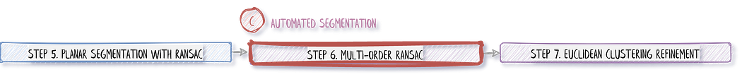
Let us frame the overall approach before approaching the project with an efficient solution. This tutorial follows a strategy comprising ten straightforward steps, as illustrated in our strategy diagram below.

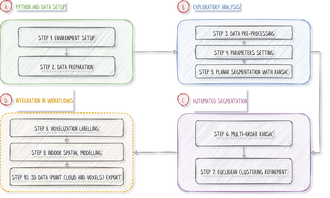
The strategy is laid out, and below, you can find the quick links to the different steps:

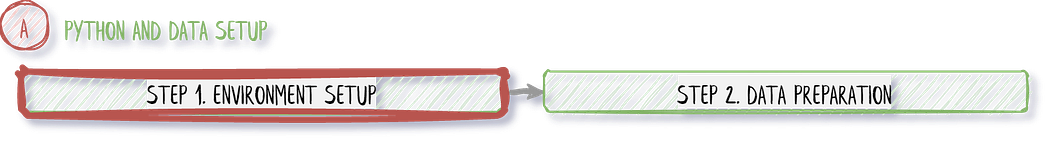
Step 1. Environment Setup
Step 2. 3D Data Preparation
Step 3. Data Pre-Processing
Step 4. Parameter Setting
Step 5. RANSAC Planar Detection
Step 6. Multi-Order RANSAC
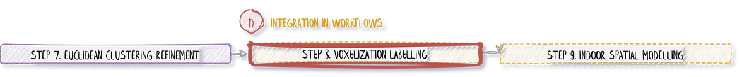
Step 7. Euclidean Clustering Refinement
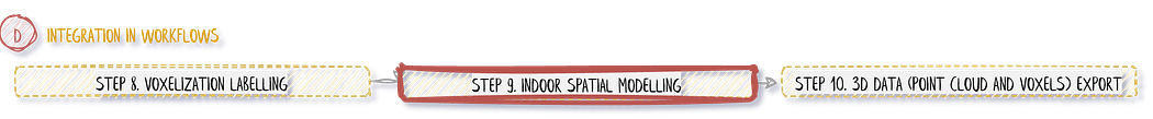
Step 8. Voxelization Labelling
Step 9. Indoor Spatial Modelling
Step 10. 3D Workflow Export

Now that we are set up, let us jump right in.

1. Set up your Python environment.

🦊 Florent: I highly recommend using a desktop setup or IDE and avoiding Google Colab IF you need to visualize 3D point clouds using the libraries provided, as they will be unstable at best or not working at worse (unfortunately…).

🤠 Ville: We guess that you are running on Windows? This is fine, but if you want to get into computational methods, Linux is the go-to choice!

Well, we will take a “parti-pris” to quickly get results. Indeed, we will accomplish excellent segmentation by following a minimalistic approach to coding 💻. That means being very picky about the underlying libraries! We will use three very robust ones, namely. numpy, matplotlib, and open3d.

Okay, to install the library package above in a fresh virtual environment, we suggest you run the following command from the cmd terminal:conda install numpy
conda install matplotlib
pip install open3d==0.16.0

🍜 Disclaimer Note: We choose Python, not C++ nor Julia, so performances are what they are 😄. Hopefully, it will be enough for your application 😉, for what we call “offline” processes (not real-time).

Within your Python IDE, make sure to import the three libraries that will be under heavy use:

#%% 1. Library setup
import numpy as np
import open3d as o3d
import matplotlib.pyplot as plt

And that is it! We are ready to rock indoor point cloud modeling workflows!

2. Point Cloud Data Preparation

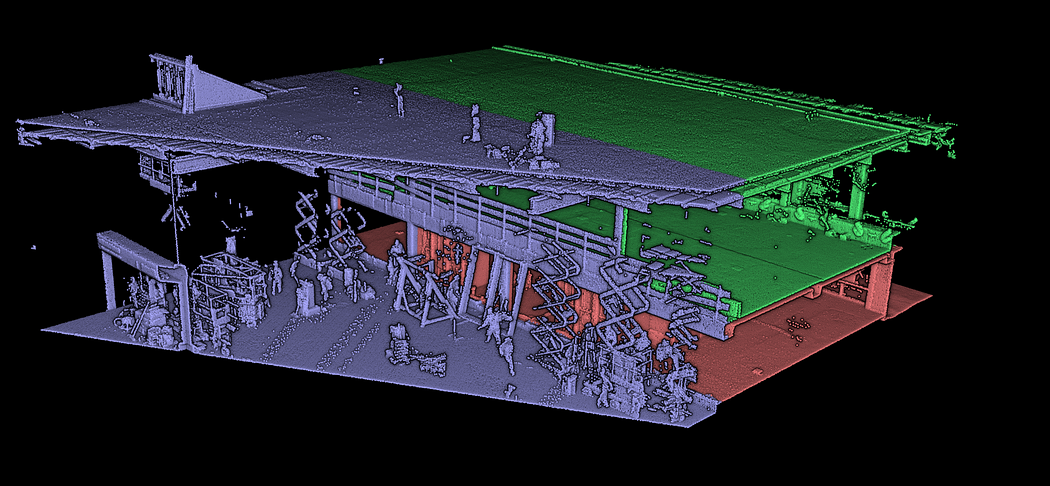
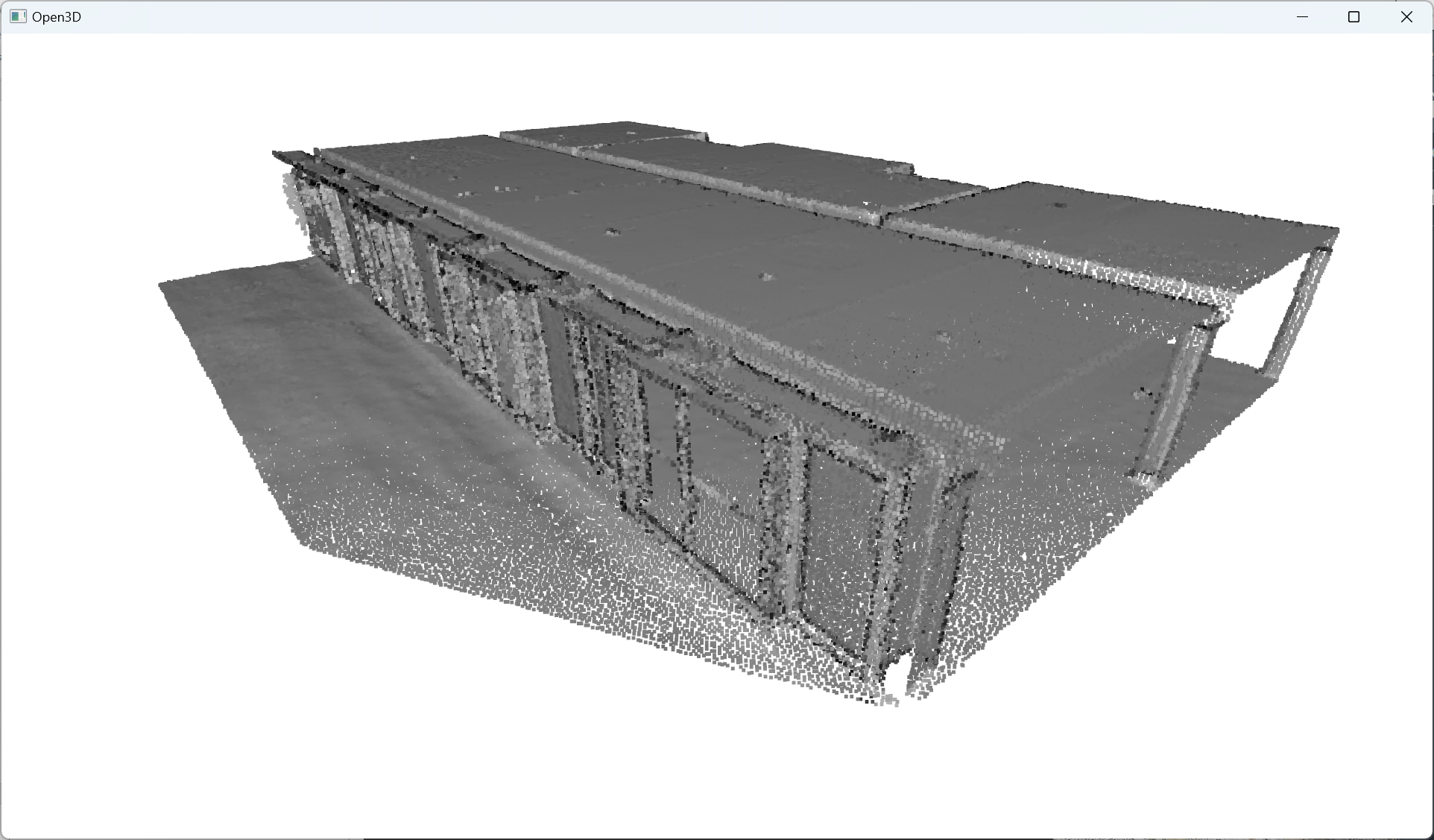
In previous tutorials, we illustrated point cloud processing and meshing over a 3D dataset obtained using an aerial LiDAR from the AHN4 LiDAR Campaign. This time, we will use a dataset gathered using a Terrestrial Laser Scanner: the ITC new building. It was organized into three different sets for you to experiment on. In purple, you have an outdoor part. In red is the ground level, and in green is the first floor, as illustrated below.

You can download the data from the Drive Folder here: ITC Datasets. Once you have a firm grasp on the data locally, you can load the dataset in your Python execution runtime with two simple lines:

DATANAME = “ITC_groundfloor.ply”
pcd = o3d.io.read_point_cloud(“../DATA/” + DATANAME)

🦊 Florent: This Python code snippet uses the Open3D library to read a point cloud data file ITC_groundfloor.ply located in the directory. “../DATA/” and assign it to the variable pcd.

The variable now holds your point cloud pcd you will play with the following:

Once the point cloud data has been successfully loaded using Open3D, the next step is to apply various pre-processing techniques to enhance its quality and extract meaningful information.

3. Point Cloud Pre-Processing

If you intend on visualizing the point cloud within open3dIt is good practice to shift your point cloud to bypass the large coordinates approximation, which creates shaky visualization effects. To apply such a shift to your pcd point cloud, first get the center of the point cloud, then translate it by subtracting it from the original variable:

pcd_center = pcd.get_center()
pcd.translate(-pcd_center)

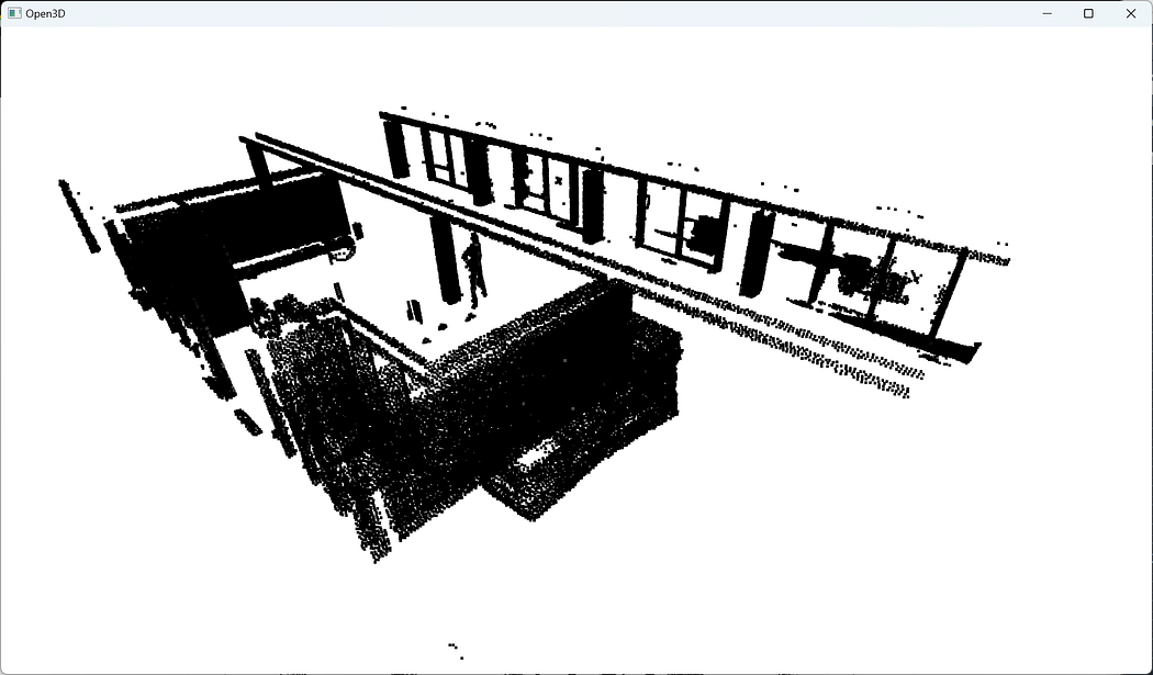
Which can now be interactively visualized with the following line of code:o3d.visualization.draw_geometries([pcd])

🦚 Note: o3d.visualization.draw_geometries([pcd]) calls the draw_geometries() function from the visualization Module in Open3D. The function takes a list of geometries as an argument and displays them in a visualization window. In this case, the list contains a single geometry, which is the pcd variable representing the point cloud. The draw_geometries() function creates a 3D visualization window and renders the point cloud. You can interact with the visualization window to rotate, zoom, and explore the point cloud from different perspectives.

Great👌, we are all set up to test some sampling strategies to unify our downward processes.

3.1. Point Cloud Random Sampling

Let us consider random sampling methods that can effectively reduce point cloud size while preserving overall structural integrity and representativeness. If we define a point cloud as a matrix (m x n), then a decimated cloud is obtained by keeping one row out of n of this matrix :

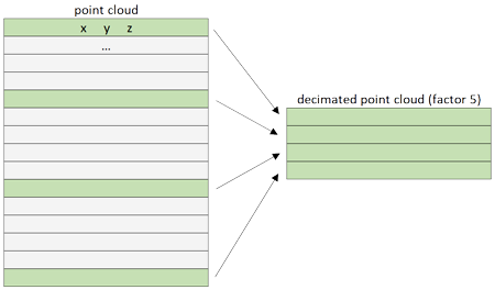
At the matrix level, the decimation acts by keeping points for every n-th row depending on the n factor. Of course, this is made based on how the points are stored in the file. Slicing a point cloud with open3d It is pretty straightforward. To shorten and parametrize the expression, you can write the lines:retained_ratio = 0.2
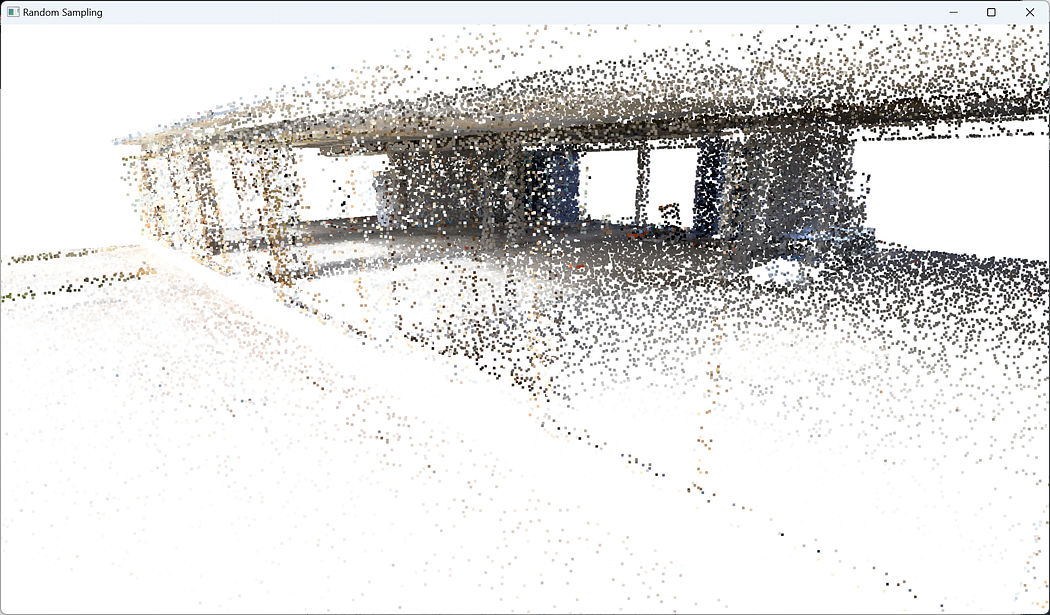
sampled_pcd = pcd.random_down_sample(retained_ratio)

🦚 Note: sampled_pcd = pcd.random_down_sample(retained_ratio) applies random downsampling to the original point cloud pcd using the random_down_sample() function provided by Open3D. The retained_ratio parameter determines the proportion of points to be retained after downsampling. For example, if retained_ratio it is set to 0.5, approximately 50% of the points will be randomly selected and retained in the sampled point cloud.o3d.visualization.draw_geometries([sampled_pcd], window_name = “Random Sampling”)

🌱 Growing: When studying 3D point clouds, random sampling has limitations that could result in missing important information and inaccurate analysis. It doesn’t consider the spatial component or relationships between the points. Therefore, it’s essential to use other methods to ensure a more comprehensive analysis.

While this strategy is quick, random sampling may not be most adapted to a “standardization” use case. The next step is to address potential outliers through statistical outlier removal techniques, ensuring the data quality and reliability for subsequent analysis and processing.

3.2. Statistical outlier removal

Using an outlier filter on 3D point cloud data can help identify and remove any data points significantly different from the rest of the dataset. These outliers could result from measurement errors or other factors that can skew the analysis. By removing these outliers, we can get a more valid representation of the data and better adjust algorithms. However, we need to be careful not to delete valuable points.

We will define a statistical_outlier_removal filter to remove points that are further away from their neighbors compared to the average for the point cloud. It takes two input parameters:

• nb_neighbors, which specifies how many neighbors are considered to calculate the average distance for a given point.
• std_ratio, which allows setting the threshold level based on the standard deviation of the average distances across the point cloud. The lower this number, the more aggressive the filter will be.

This amount to the following:nn = 16
std_multiplier = 10

filtered_pcd, filtered_idx = pcd.remove_statistical_outlier(nn, std_multiplier)

🦚 Note: the remove_statistical_outlier() the function applies statistical outlier removal to the point cloud using a specified number of nearest neighbors (nn) and a standard deviation multiplier (std_multiplier). The function returns two values: filtered_pcd and filtered_idx. filtered_pcd represents the filtered point cloud, where statistical outliers have been removed. filtered_idx is an array of indices corresponding to the points in the original point cloud pcd that were retained after the outlier removal process.

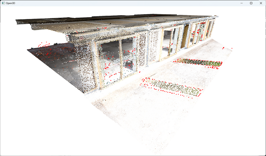
To visualize the results of this filtering technique, we color the outliers in red and add them to the list of point cloud objects we want to visualize:outliers = pcd.select_by_index(filtered_idx, invert=True)
outliers.paint_uniform_color([1, 0, 0])
o3d.visualization.draw_geometries([filtered_pcd, outliers])

After removing statistical outliers from the point cloud, the next step involves applying voxel-based sampling techniques to downsample the data further, facilitating efficient processing and analysis while preserving the essential structural characteristics of the point cloud.

3.3. Point Cloud Voxel (Grid) Sampling

The grid subsampling strategy is based on the division of the 3D space in regular cubic cells called voxels. For each cell of this grid, we only keep one representative point, and this point, the representative of the cell, can be chosen in different ways. When subsampling, we keep that cell’s closest point to the barycenter.

Concretely, we define a voxel_size that we then use to filter our point cloud:voxel_size = 0.05
pcd_downsampled = filtered_pcd.voxel_down_sample(voxel_size = voxel_size)

🦚 Note: This line performs voxel downsampling on the filtered point cloud, filtered_pcd, using the voxel_down_sample() function. The voxel_size parameter specifies the size of each voxel for downsampling the point cloud. Larger voxel sizes result in a more significant reduction in point cloud density. The result of the downsampling operation is assigned to the variable pcd_downsampled, representing the downsampled point cloud.

Time to visualize the repartition closely after our downsampling:o3d.visualization.draw_geometries([pcd_downsampled])

At this stage, we have an outlier point set left untouched in further processing and a downsampled point cloud that constitutes the new subject of the subsequent processes.

3.4. Point Cloud Normals Extraction

A point cloud normal refers to the direction of a surface at a specific point in a 3D point cloud. It can be used for segmentation by dividing the point cloud into regions with similar normals, for example. In our case, normals will help identify objects and surfaces within the point cloud, making it easier to visualize. And it is an excellent opportunity to introduce a way to compute such normals semi-automatically. We first define the average distance between each point in the point cloud and its neighbors:nn_distance = 0.05

Then we use this information to extract a limited max_nn points within a radius radius_normals to compute a normal for each point in the 3D point cloud:radius_normals=nn_distance*4
pcd_downsampled.estimate_normals(search_param=o3d.geometry.KDTreeSearchParamHybrid(radius=radius_normals, max_nn=16), fast_normal_computation=True)

The pcd_downsampled point cloud object is now proud to have normals, ready to display its prettiest side 😊. You know the drill at this stage:

pcd_downsampled.paint_uniform_color([0.6, 0.6, 0.6])
o3d.visualization.draw_geometries([pcd_downsampled,outliers])

Upon completing the voxel downsampling of the point cloud, the subsequent step involves configuring the parameters for point cloud shape detection and clustering, which plays a crucial role in grouping similar points together and extracting meaningful structures or objects from the downsampled point cloud data.

4. Point Cloud Parameter setting for 3D Shape Detection

In this tutorial, we have selected two of the most effective and reliable methods for 3D Shape detection and clustering for you to master: RANSAC and Euclidean Clustering using DBSCAN. However, before utilizing these approaches, hence understanding the parameters, it is crucial to comprehend the fundamental concepts in simple terms.

RANSAC

The RANSAC algorithm, short for RANdom SAmple Consensus, is a powerful tool for handling data that contains outliers, which is often the case when working with real-world sensors. The algorithm works by grouping data points into two categories: inliers and outliers. By identifying and ignoring the outliers, you can focus on working with reliable inliers, making your analysis more effective.

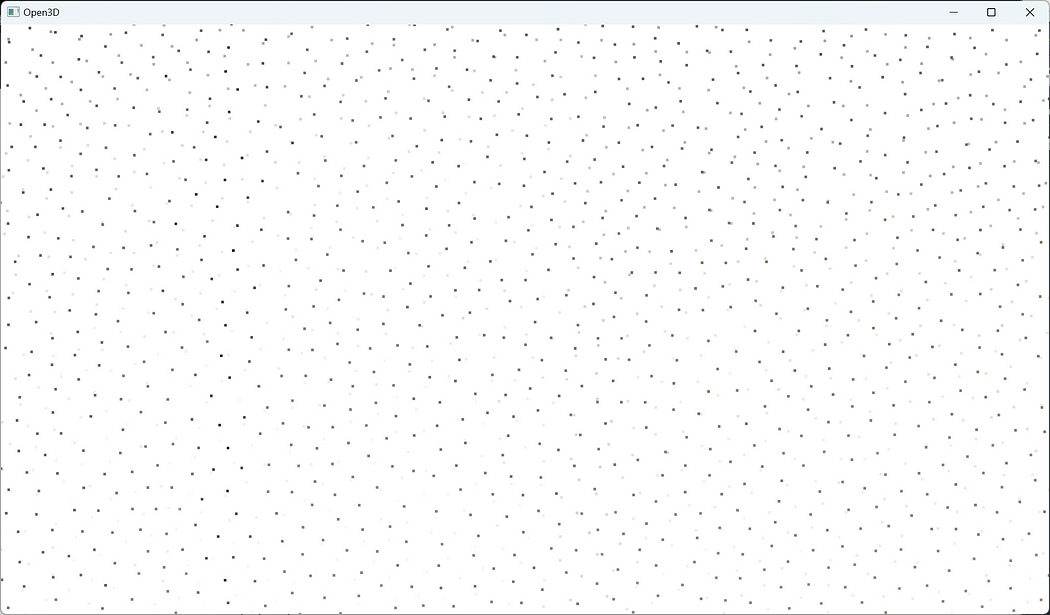
So let me use a tiny but simple example to illustrate how RANSAC works. Let us say that we want to fit a plane through the point cloud below. How can we do that?

First, we create a plane from the data, and for this, we randomly select 3 points from the point cloud necessary to establish a plane. And then, we simply check how many of the remaining points kind of fall on the plane (to a certain threshold), which will give a score to the proposal.

Then, we repeat the process with 3 new random points and see how we are doing. Is it better? Is it worse? And again, we repeat this process over and over again, let’s say 10 times, 100 times, 1000 times, and then we select the plane model with the highest score (i.e. which has the best “support” of the remaining data points). And that will be our solution: the supporting points plus the three points that we have sampled constitute our inlier point set, and the rest is our outlier point set. Easy enough, hun 😁?

Haha, but for the skeptics, don’t you have a rising question? How do we actually determine how many times we should repeat the process? How often should we try that? Well, that is actually something that we can compute, but let’s put it aside, for now, to focus on the matter at hand: point cloud segmentation 😉.

RANSAC Parameter Setting

We want to use RANSAC for detecting 3D planar shapes in our point cloud. To use RANSAC, we need to define three parameters: a distance threshold distance_threshold that allows tagging a point inlier or outlier to the 3D shape; a minimal number of point ransac_n selected to fit the geometric model; a number of iterations num_iterations.

Determination of the Distance threshold: We may be a bit limited by needing some domain knowledge to set up future segmentation and modeling threshold. Therefore, it would be exciting to try and bypass this to open the approach to non-experts. we will share with you a straightforward thought that could be useful. What if we were to compute the mean distance between points in our datasets and use this as a base to set up our threshold?

Well, it is an idea worth exploring. To determine such a value, we use a KD-Tree to speed up the process of querying the nearest neighbors for each point. From there, we can then query the k-nearest neighbors for each point in the point cloud, which is then packed in the open3d function shown below:nn_distance = np.mean(pcd.compute_nearest_neighbor_distance())

without much surprise, it is close to 5 cm as we sampled our point cloud to this value. It means that if we reasoned by considering the nearest neighbor, we would have an average distance of 51 mm.

🌱 Growing: From there, what we could do it to set the RANSAC parameter to a value derived from the nn_distance variable, which would then be adapted to the considered dataset, independently from domain knowledge. How would you approach this?

Determination of the point number: Here, it is quick. We want to find planes, so we will take the minimum number of points needed to define a 3D plane: 3.

Determination of the iteration number: The more iteration you have, the more robust your 3D shape detection works, but the longer it takes. For now, we can leave that to 1000, which yields good results. We will explore more ingenious ways to find the noise ratio of a point cloud in future tutorials. 😉

🧙‍♂️ Experts: There exists an automatic way to get the iteration number right every time. If we want to succeed with a probability p (e.g., 99%), the outlier ratio in our data is e (e.g., 60%), and we need s point to define our model (here 3). The formula below gives us the expected number of iterations:

Now that our RANSAC parameters are defined, we can study a first segmentation pass.

5. Point Cloud Segmentation with RANSAC

Let us first set the different thresholds to non-automatic values for testing:

distance_threshold = 0.1
ransac_n = 3
num_iterations = 1000

From there, we can segment the point cloud using RANSAC to detect planes with the following lines:

plane_model, inliers = pcd.segment_plane(distance_threshold=distance_threshold,ransac_n=3,num_iterations=1000)
[a, b, c, d] = plane_model
print(f”Plane equation: {a:.2f}x + {b:.2f}y + {c:.2f}z + {d:.2f} = 0″)

We gather results in two variables: plane_model, which holds the parameters a,b,c,d of a plane, and the inliers as point indexes.

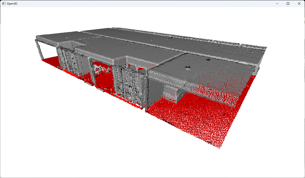
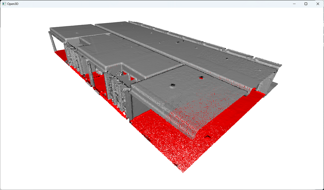
This allows to use the indexes to segment the point cloud in a inlier_cloud point set (that we color in red), and outlier_cloud point set (that we color in grey:

inlier_cloud = pcd.select_by_index(inliers)
outlier_cloud = pcd.select_by_index(inliers, invert=True)

#Paint the clouds
inlier_cloud.paint_uniform_color([1.0, 0, 0])
outlier_cloud.paint_uniform_color([0.6, 0.6, 0.6])

#Visualize the inliers and outliers
o3d.visualization.draw_geometries([inlier_cloud, outlier_cloud])

🦊 Florent: The argument invert=True permits to select the opposite of the first argument, which means all indexes not present in inliers. If you are lacking the shading, remember to compute the normals, as shown above.

🌱 Growing: Try and adjust the various parameters, and study the impact with a qualitative analysis. Remember first to decorrelate changes (one variable at a time); else your analysis may be biased 😊.

Great! You know how to segment your point cloud in an inlier point set and an outlier point set 🥳! Now, let us study how to find some clusters close to one another. So let us imagine that once we detected the big planar portions, we have some “floating” objects that we want to delineate. How to do this? (yes, it is a false question, we have the answer for you 😀)

6. Scaling 3D Segmentation: Multi-Order RANSAC

Our philosophy will be very simple. We will first run RANSAC multiple times (let say n times) to extract the different planar regions constituting the scene. Then we will deal with the “floating elements” through Euclidean Clustering (DBSCAN). It means that we have to make sure we have a way to store the results during iterations. Ready?

Okay, let us instantiate an empty dictionary that will hold the results of the iterations (the plane parameters in segment_models, and the planar regions from the point cloud in segments):segment_models={}
segments={}

Then, we want to make sure that we can influence later on the number of times we want to iterate for detecting the planes. To this end, let us create a variable max_plane_idx that holds the number of iterations:max_plane_idx=10

🦊 Florent: Here, we say that we want to iterate 10 times to find 10 planes, but there are smarter ways to define such a parameter. It actually extends the scope of the article and will be covered in another session.

Now let us go into a working loopy-loopy 😁, that I will first quickly illustrate.

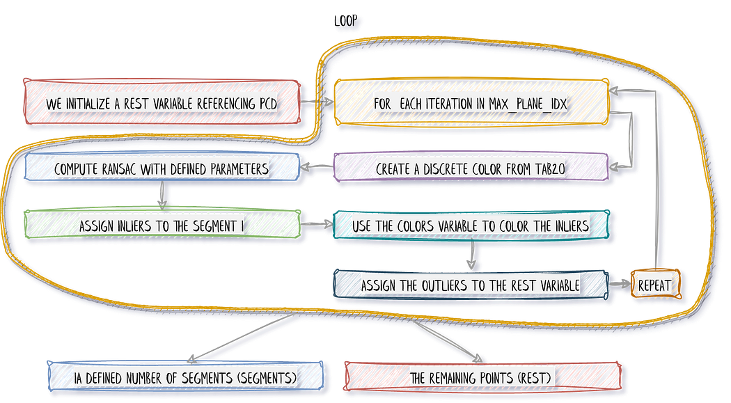
In the first pass (loop i=0), we separate the inliers from the outliers. We store the inliers in segments, and then we want to pursue with only the remaining points stored in rest, that becomes the subject of interest for the loop n+1 (loop i=1). That means that we want to consider the outliers from the previous step as the base point cloud until reaching the above threshold of iterations (not to be confused with RANSAC iterations). This translates into the following:

rest=pcd
for i in range(max_plane_idx):
colors = plt.get_cmap(“tab20”)(i)
segment_models[i], inliers = rest.segment_plane(
distance_threshold=0.1,ransac_n=3,num_iterations=1000)
segments[i]=rest.select_by_index(inliers)
segments[i].paint_uniform_color(list(colors[:3]))
rest = rest.select_by_index(inliers, invert=True)
print(“pass”,i,”/”,max_plane_idx,”done.”)

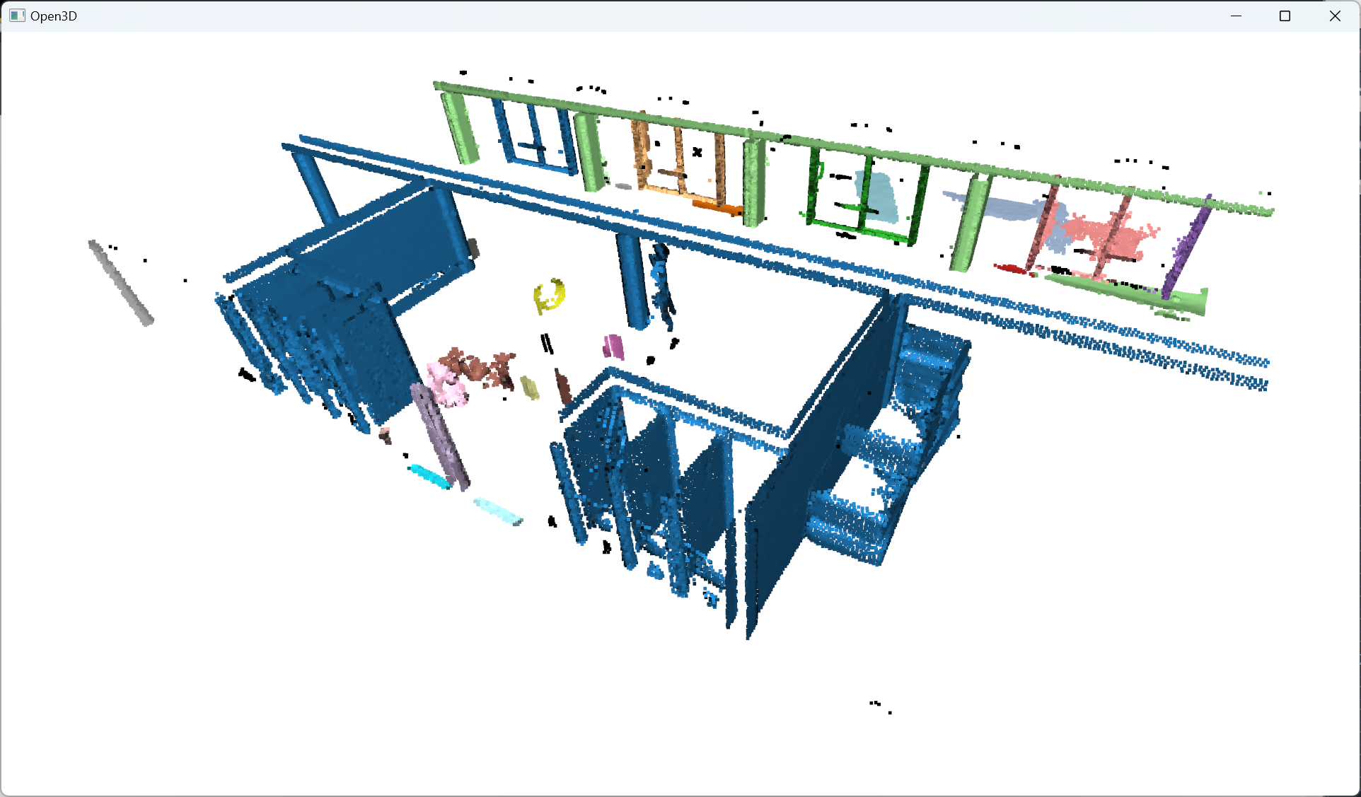
And that is pretty much it! Now, for visualizing the ensemble, as we paint each segment detected with a color from tab20 through the first line in the loop (colors = plt.get_cmap("tab20")(i)), you just need to write:o3d.visualization.draw_geometries([segments[i] for i in range(max_plane_idx)]+[rest])

🦚 Note: The list [segments[i] for i in range(max_plane_idx)] that we pass to the function o3d.visualization.draw_geometries() is actually a “list comprehension” 🤔. It is equivalent to writing a for loop that appends the first element segments[i] to a list. Conveniently, we can then add the [rest] to this list and the draw.geometries() method will understand we want to consider one point cloud to draw. How cool is that?

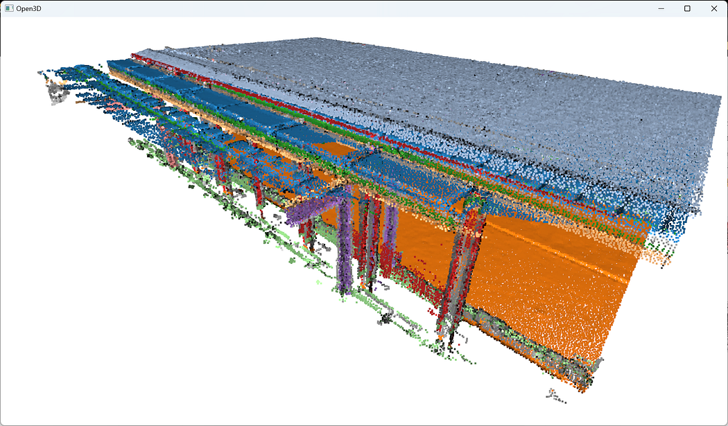
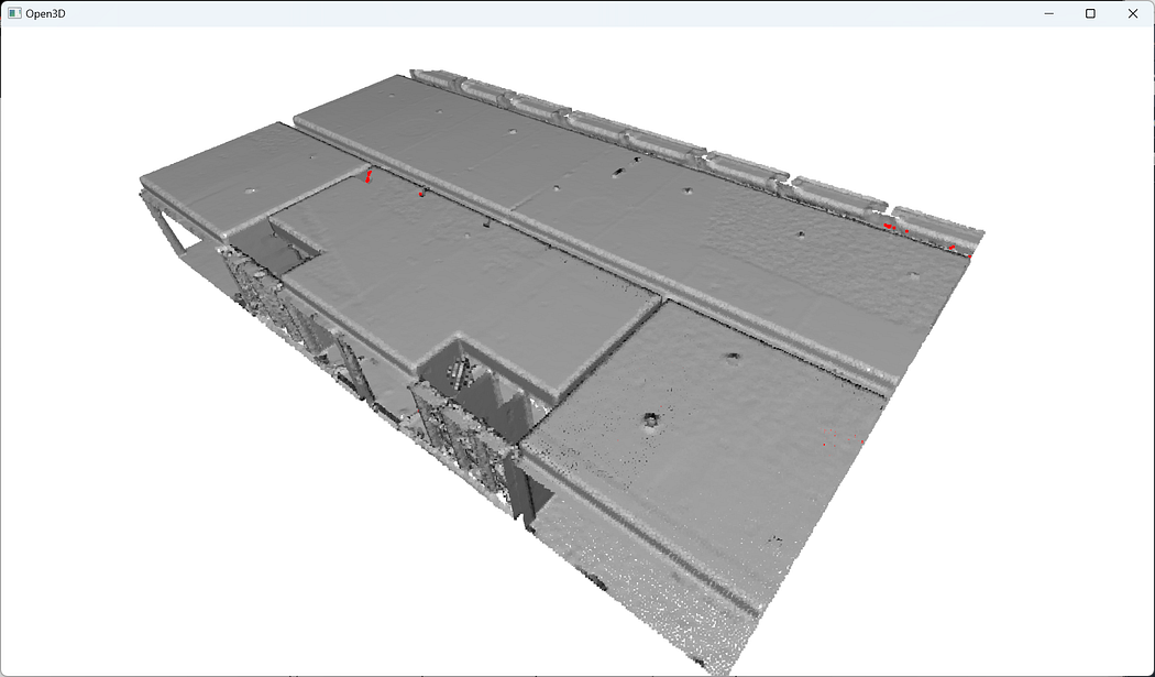
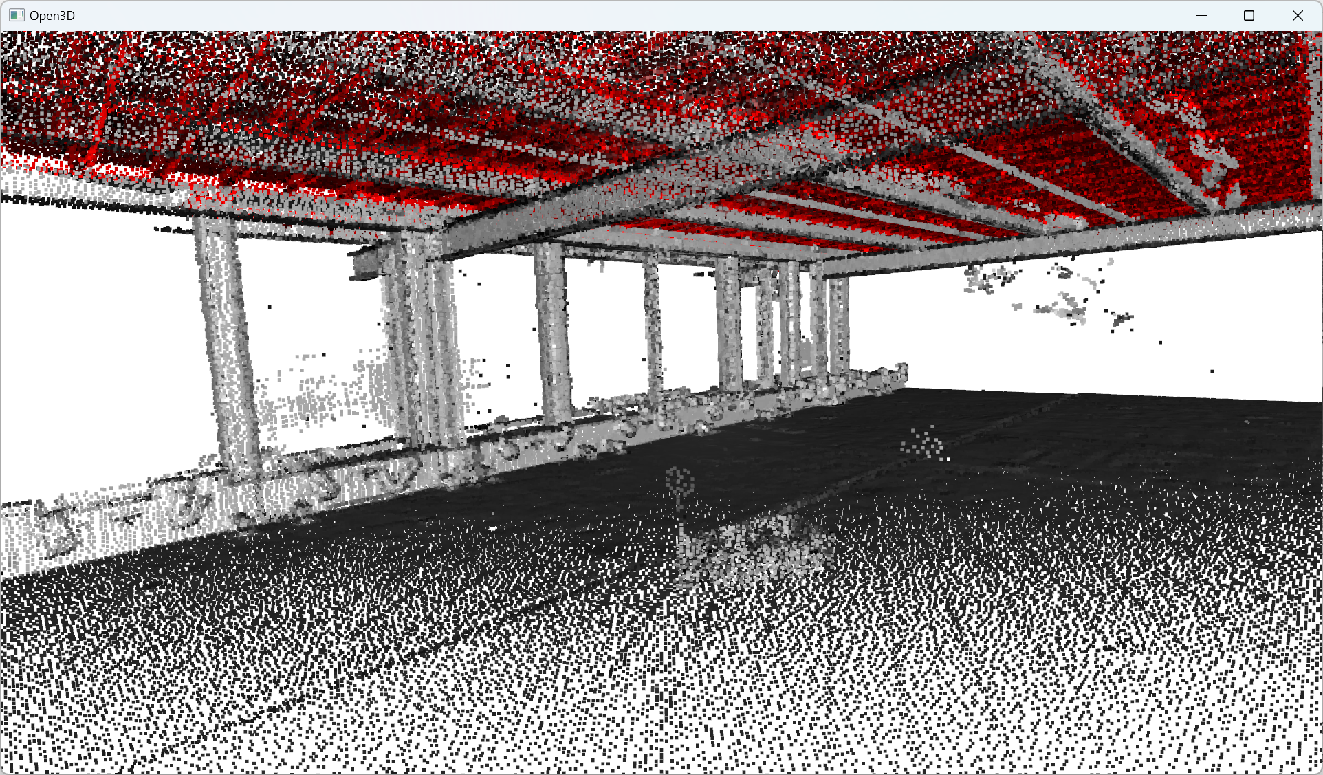
Ha! We think we are done… But are we? Do you notice something strange here? If you look closely, there are some strange artifacts, like “red lines/planes” that actually cut some planar elements. Why? 🧐

In fact, because we fit all the points to RANSAC plane candidates (which have no limit extent in the Euclidean space) independently of the point’s density continuity, then we have these “lines” artifacts depending on the order in which the planes are detected. So the next step is to prevent such behavior! For this, I propose to include in the iterative process a condition based on Euclidean clustering to refine inlier point sets in contiguous clusters. To this end, we will rely on the DBSCAN algorithm.

Euclidean Clustering (DBSCAN)

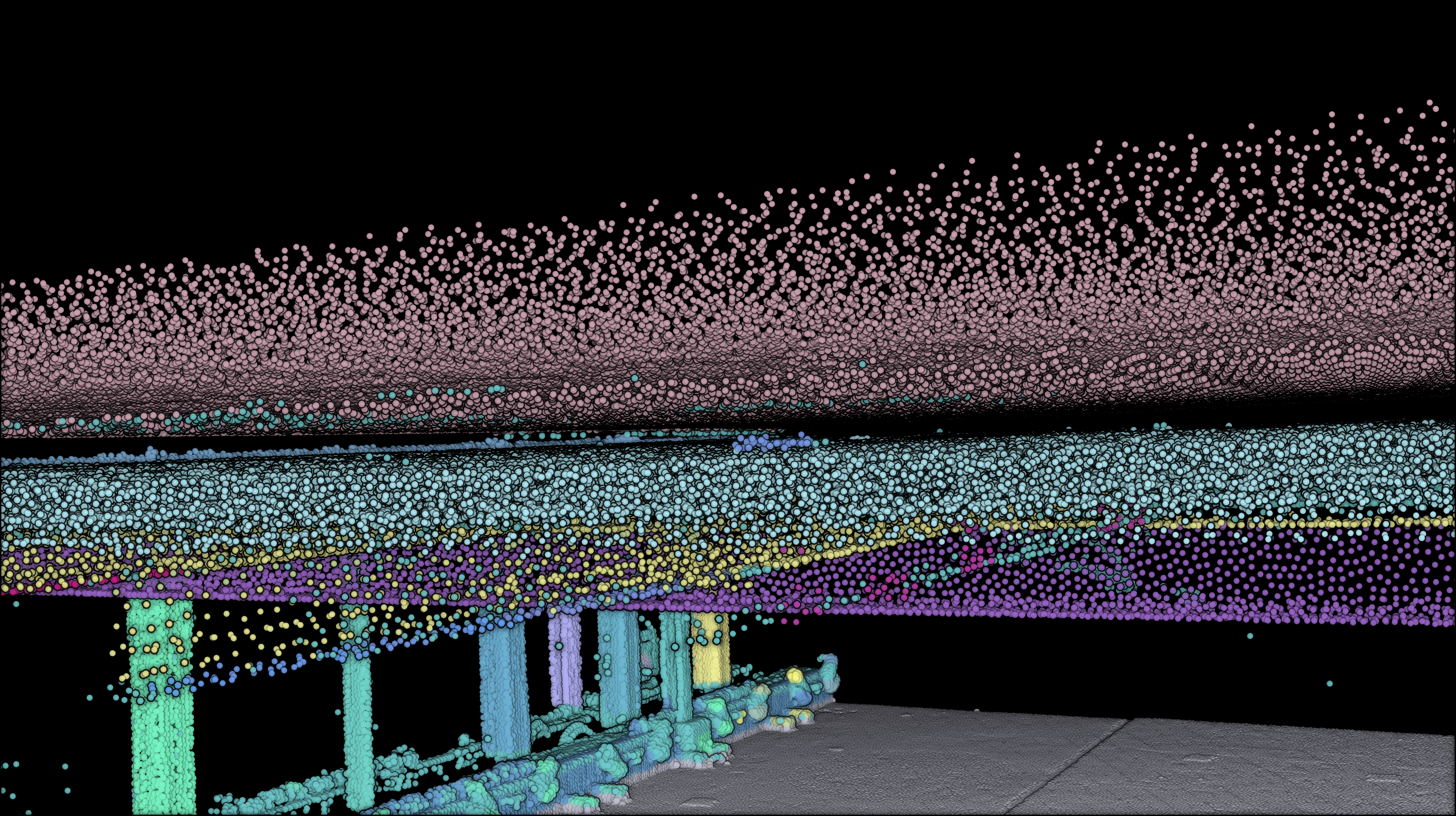
With point cloud datasets, we often need to group sets of points spatially contiguous (i.e. that are physically close or adjacent to each other in 3D space), as illustrated below. But how can we do this efficiently?

The DBSCAN (Density-Based Spatial Clustering of Applications with Noise) algorithm was introduced in 1996 for this purpose. This algorithm is widely used, which is why it was awarded a scientific contribution award in 2014 that has stood the test of time.

The DBSCAN algorithm involves scanning through each point in the dataset and constructing a set of reachable points based on density. This is achieved by analyzing the neighborhood of each point and including it in the region if it contains enough points. The process is repeated for each neighboring point until the cluster can no longer expand. Points that do not have enough neighbors are labeled as noise, making the algorithm robust to outliers. It’s pretty impressive, isn’t it? 😆

Ah, we almost forgot. The choice of parameters (ϵ for the neighborhood and n_min for the minimal number of points) can also be tricky: One must take great care when setting parameters to create enough interior points (which will not happen if n_min is too large or ϵ too small). In particular, this means that DBSCAN will have trouble finding clusters of different densities. BUT, DBSCAN has the great advantage of being computationally efficient without requiring to predefine the number of clusters, unlike Kmeans, for example. Finally, it allows for finding clusters of arbitrary shapes. We are now ready to dive in the parameter dark side of things 💻

DBSCAN for 3D Point Cloud Clustering

Let me detail the logical process (Activate the beast mode👹). First, we need to define the parameters to run DBSCAN:epsilon = 0.15
min_cluster_points = 5

🌱 Growing: The definition of these parameters is something to explore. You have to find a way to balance over-segmentation and under-segmentation problematics. Eventually, you can use some heuristics determination based on the initial distance definition of RANSAC. Something to explore 😉.

Within the for loop that we defined before, we will run DBSCAN just after the assignment of the inliers (segments[i]=rest.select_by_index(inliers)), by adding the following line right after:labels = np.array(segments[i].cluster_dbscan(eps=epsilon, min_points=min_cluster_points))

Then, we will count how many points each cluster that we found holds, using a weird notation that makes use of a list comprehension. The result is then stored in the variable candidates:candidates=[len(np.where(labels==j)[0]) for j in np.unique(labels)]

And now? We have to find the “best candidate”, which is normally the cluster that holds the more points! And for this, here is the line:best_candidate=int(np.unique(labels)[np.where(candidates== np.max(candidates))[0]])

Okay, many tricks are happening under the hood here, but essentially, we use our Numpy proficiency to search and return the index of the points that belong to the biggest cluster. From here, it is downhill skiing, and we just need to ensure that we include any remaining clusters from each iteration for consideration in subsequent RANSAC iterations (🔥 recommendation to to read 5 times the sentence to digest!):

rest = rest.select_by_index(inliers, invert=True) + segments[i].select_by_index(list(np.where(labels!=best_candidate)[0]))
segments[i]=segments[i].select_by_index(list(np.where(labels== best_candidate)[0]))

🦚 Note: the rest variable now makes sure to hold both the remaining points from RANSAC and DBSCAN. And of course, the inliers are now filtered to the biggest cluster present in the raw RANSAC inlier set.

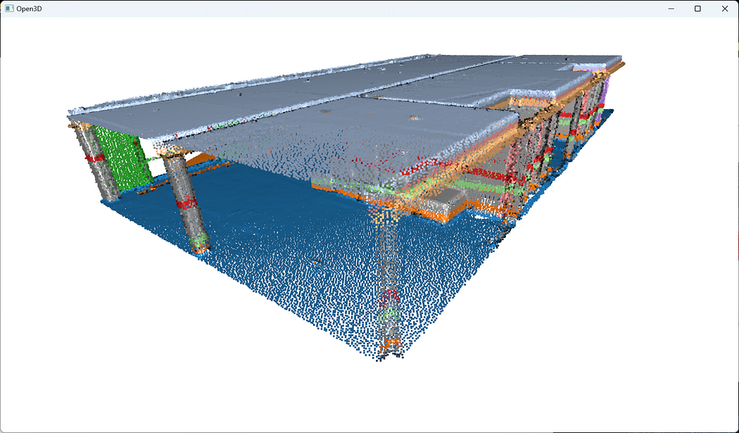
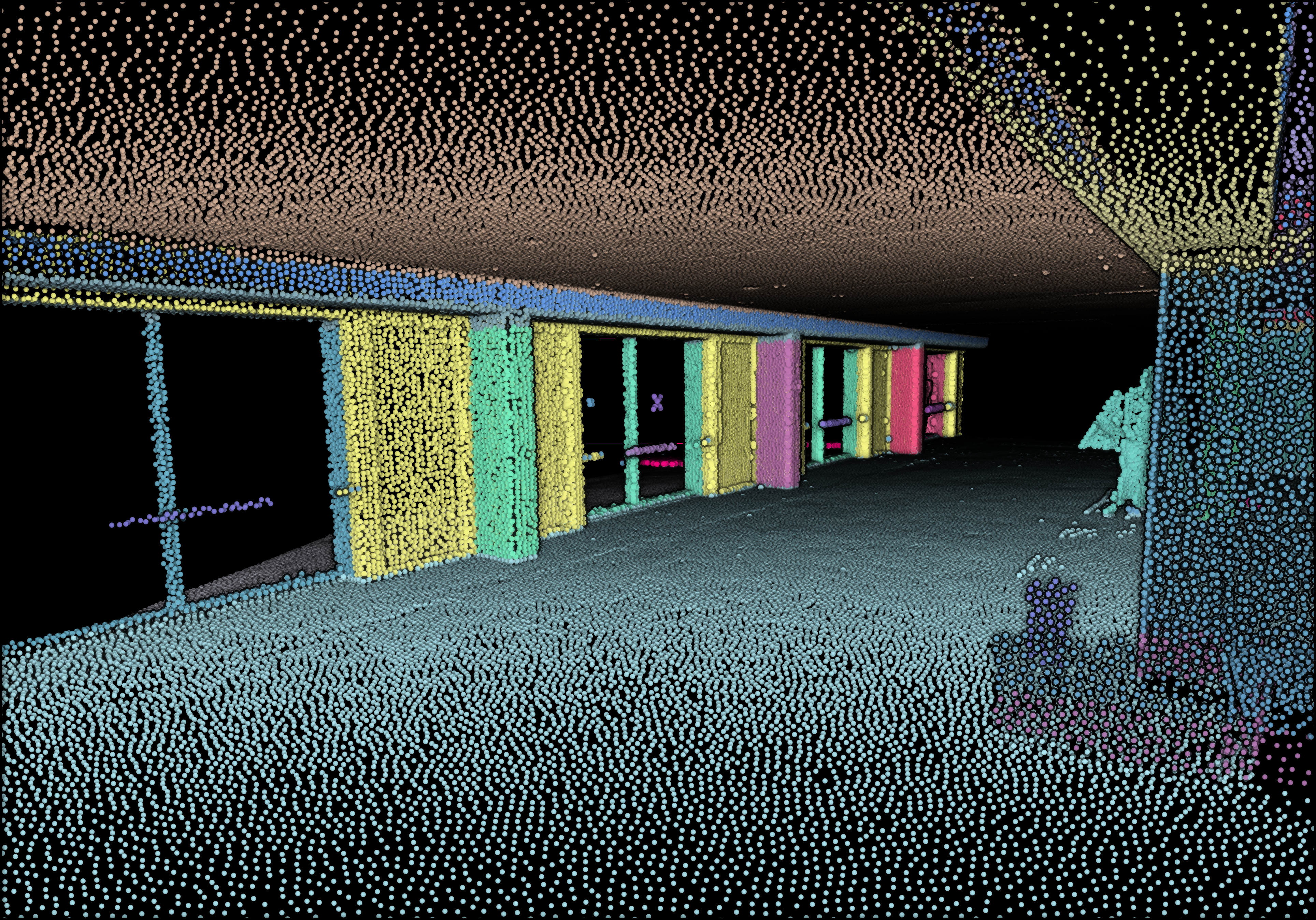
When the loop is over, you get a clean set of segments holding spatially contiguous point sets that follow planar shapes, that you can visualize with different colors using the following lines of code in the loop:

colors = plt.get_cmap(“tab20”)(i)
segments[i].paint_uniform_color(list(colors[:3]))

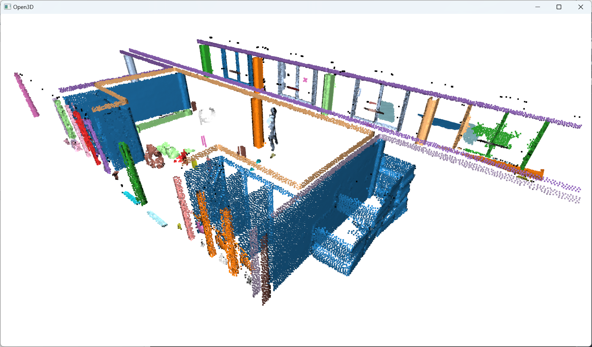
The results should be something similar to this:

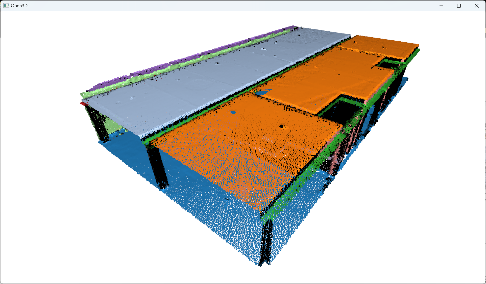
But is this the end? Noooo, never 😄! Once the multi-order RANSAC segmentation has been applied to the point cloud, the next stage involves refining the remaining non-segmented points through the utilization of DBSCAN, which aids in further enhancing the granularity of the point cloud analysis with additional clusters.

🦚 Note: Granularity is a useful academic word that is used a lot in data science. The granularity of data means the level of detail in how it is organized or modeled. Here, the smaller objects we can model from the point cloud, the finer granularity our representation has. (fancy, right?!)

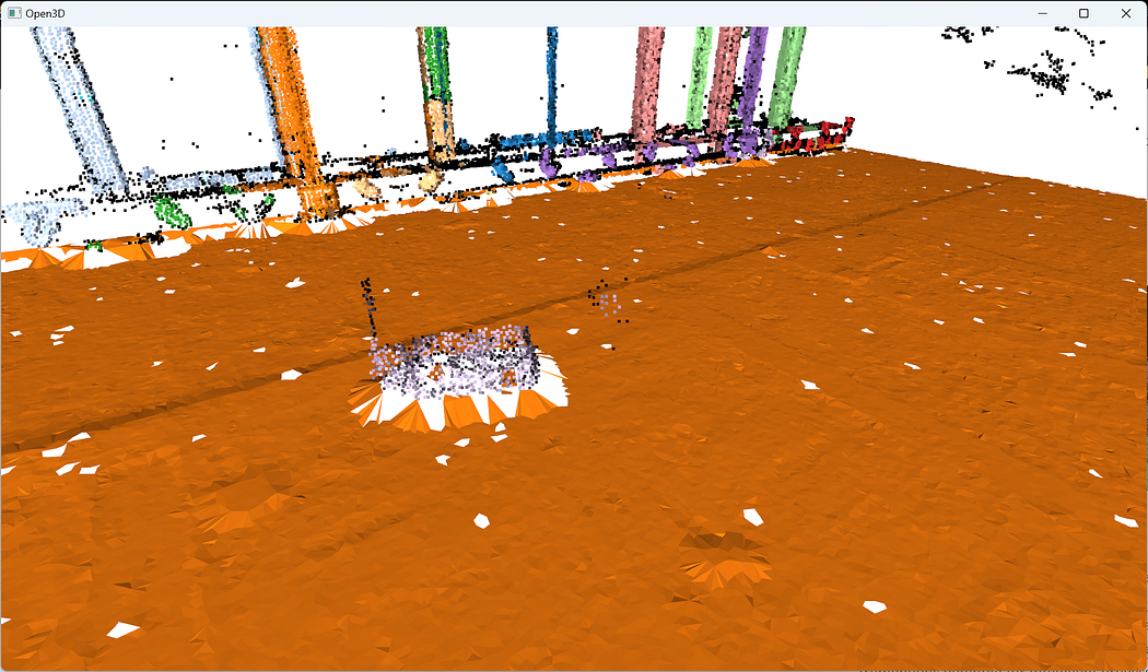
7. Euclidean Clustering Refinement for 3D Shape Detection

Okay, time to evade the loop, and work on the remaining points assigned to therest variable, that are not yet attributed to any segment. Let us first get a visual grasp on what we are talking about:o3d.visualization.draw_geometries([rest])

We can apply a simple pass of Euclidean clustering with DBSCAN and capture the results in a labels variable. You know the drill:labels = np.array(pcd.cluster_dbscan(eps=0.1, min_points=10))

🌱 Growing: We use a radius of 10 cm for “growing” clusters and consider one only if, after this step, we have at least 10 points. But is this the right choice? 🤔Feel free to experiment to find a good balance and, ideally, a way to automate this😀.

The labels vary between -1 and n, where -1 indicate it is a “noise” point and values 0 to n are then the cluster labels given to the corresponding point. Note that we want to get the labels as a NumPy array thereafter.

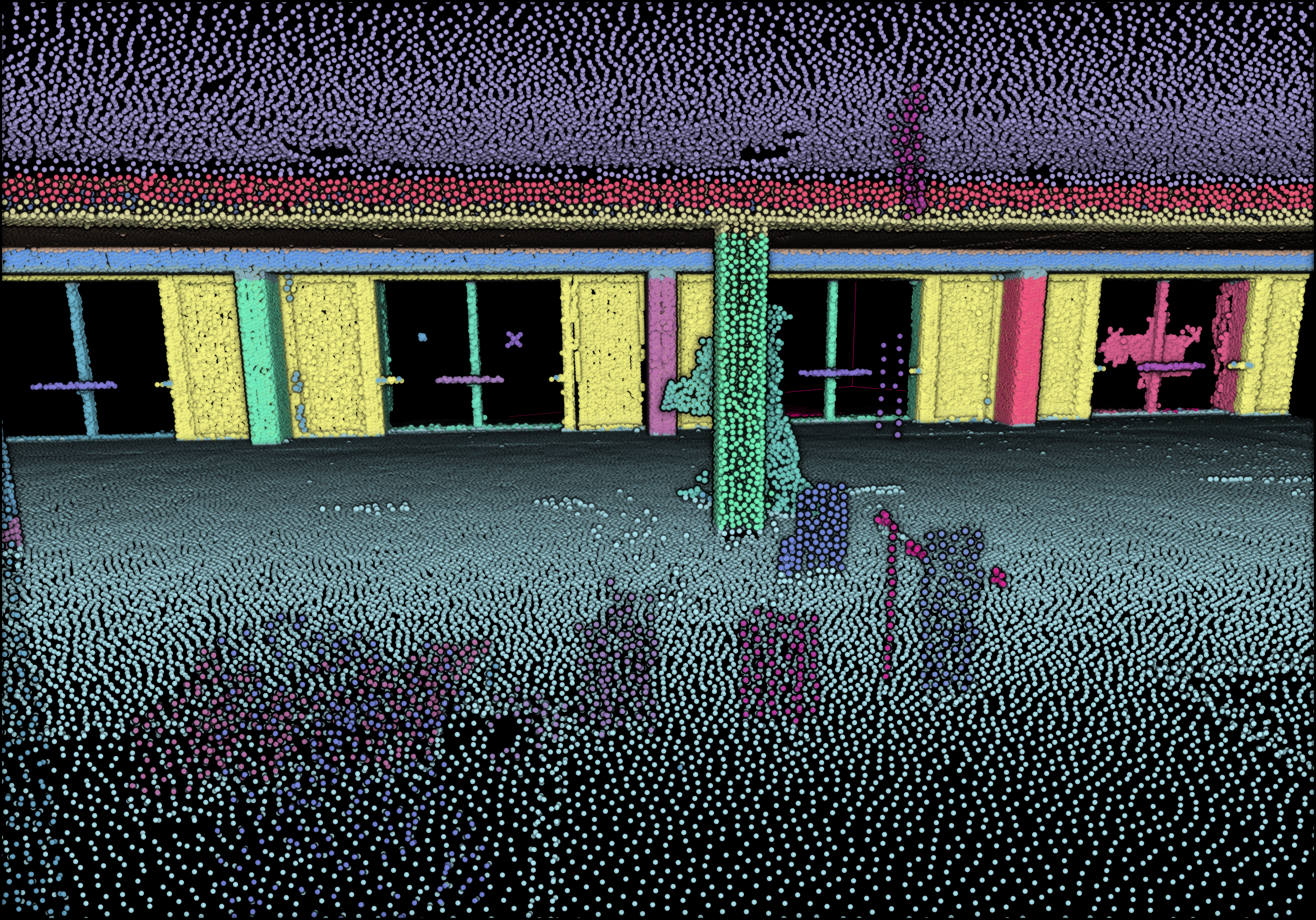
Nice. Now that we have groups of points defined with a label per point, let us color the results. This is optional, but it is handy for iterative processes to search for the right parameter’s values. To this end, we propose to use the Matplotlib library to get specific color ranges, such as the tab20:

max_label = labels.max()
colors = plt.get_cmap(“tab20”)(labels / (max_label
if max_label > 0 else 1))
colors[labels < 0] = 0
rest.colors = o3d.utility.Vector3dVector(colors[:, :3])
o3d.visualization.draw_geometries([rest])

🦚 Note: The max_label should be intuitive: it stores the maximal value in the labels list. This permits to use it as a denominator for the coloring scheme while treating with an “if” statement the special case where the clustering is skewed and delivers only noise + one cluster. After, we make sure to set these noisy points with the label -1 to black (0). Then, we give to the attribute colors of the point cloud pcd the 2D NumPy array of 3 “columns”, representing R, G, B.

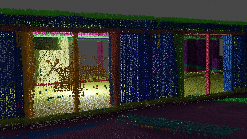
Et voilà! I employ the same methodology as before, no sorcery! I just make sure to use coherent parameters to have a refined clustering to get the beautiful rainbow scene you always dreamed of 🥳!

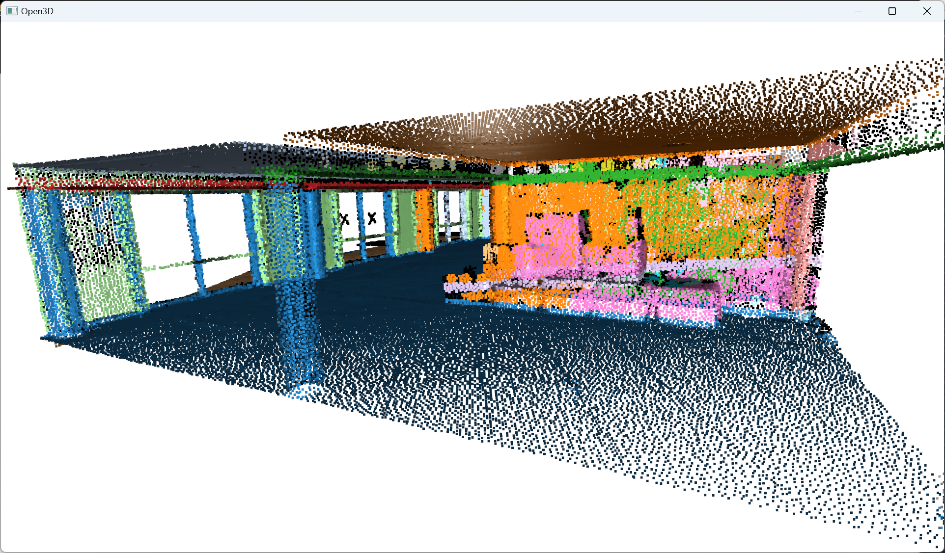
After refining the point cloud clustering results using DBSCAN, the focus shifts to the voxelization technique, which involves organizing the data into a meaningful spatial structure, thereby enabling efficient modeling of the point cloud information.

8. Voxelization and Labelling for 3D Shape Detection

Now that we have a point cloud with segment labels, it would be very interesting to see if we could fit indoor modeling workflows. One way to approach this is the use of voxels to accommodate for O-Space and R-Space. By dividing a point cloud into small cubes, it becomes easier to understand a model’s occupied and empty spaces. Let us get into it.

9.1. Voxel Grid Generation

Creating accurate and detailed 3D models of the space means generating a nice and tight voxel grid. This technique divides a point cloud into small cubes or voxels with their own coordinate system.

To create such a structure, we first define the size of our new entity: the voxel:voxel_size=0.5

Now, we want to know how many of these cubes we must stack onto one another to fill the bounding box defined by our point cloud. This means that we have first to compute the extent of our point cloud:min_bound = pcd.get_min_bound()
max_bound = pcd.get_max_bound()

Great, now we use the o3d.geometry.VoxelGrid.create_from_point_cloud() function onto any point cloud of choice to fit a voxel grid on it. but wait. Which point cloud do we want to distinguish for further processes?

Okay, let us illustrate the case where you want to have voxels of “structural” elements vs voxels of clutter that do not belong to structural elements. Without labeling, we could guide our choice based on whether or not they belong to RANSAC segments or other segments; This means first concatenating the segments from the RANSAC pass:

pcd_ransac=o3d.geometry.PointCloud()
for i in segments:
pcd_ransac += segments[i]

🦚 Note: At this stage, you have the ability to color the point clouds with a uniform color later picked up by the voxels. If this is something you would like, you can use: pcd_ransac.paint_uniform_color([1, 0, 0])

Then, we can simply extract our voxel grid:voxel_grid_structural = o3d.geometry.VoxelGrid.create_from_point_cloud(pcd_ransac, voxel_size=voxel_size)

and do the same thing for the remaining elements:

rest.paint_uniform_color([0.1, 0.1, 0.8])
voxel_grid_clutter = o3d.geometry.VoxelGrid.create_from_point_cloud(rest, voxel_size=voxel_size)

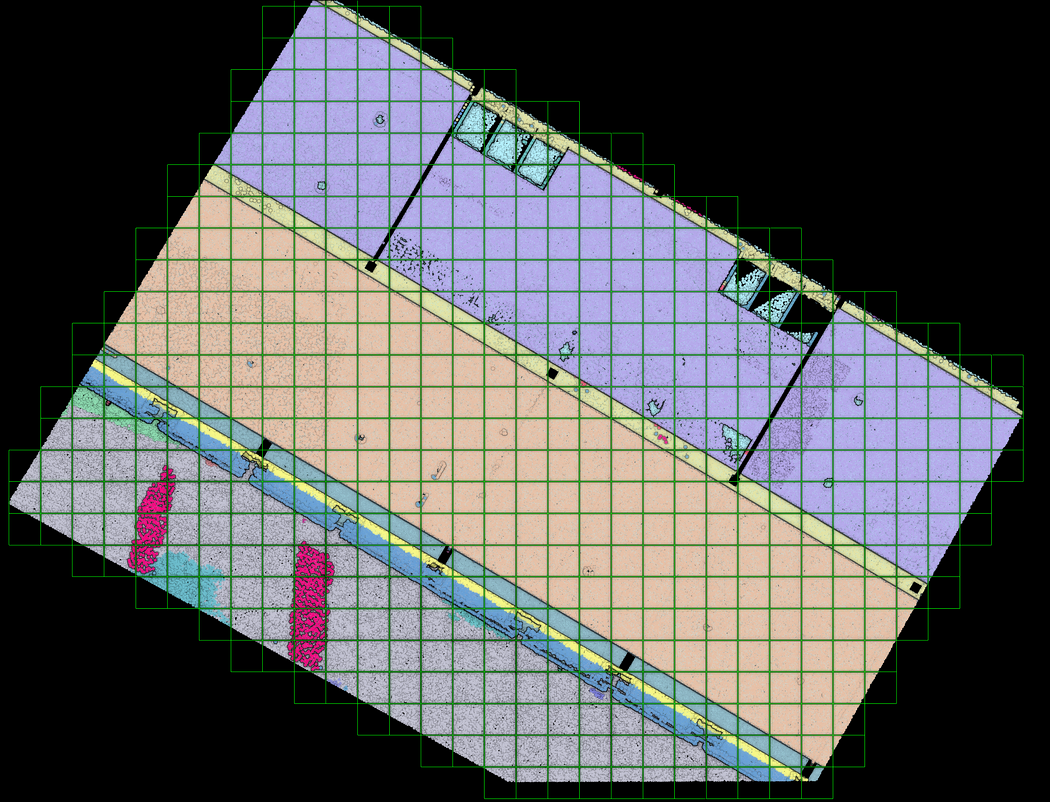
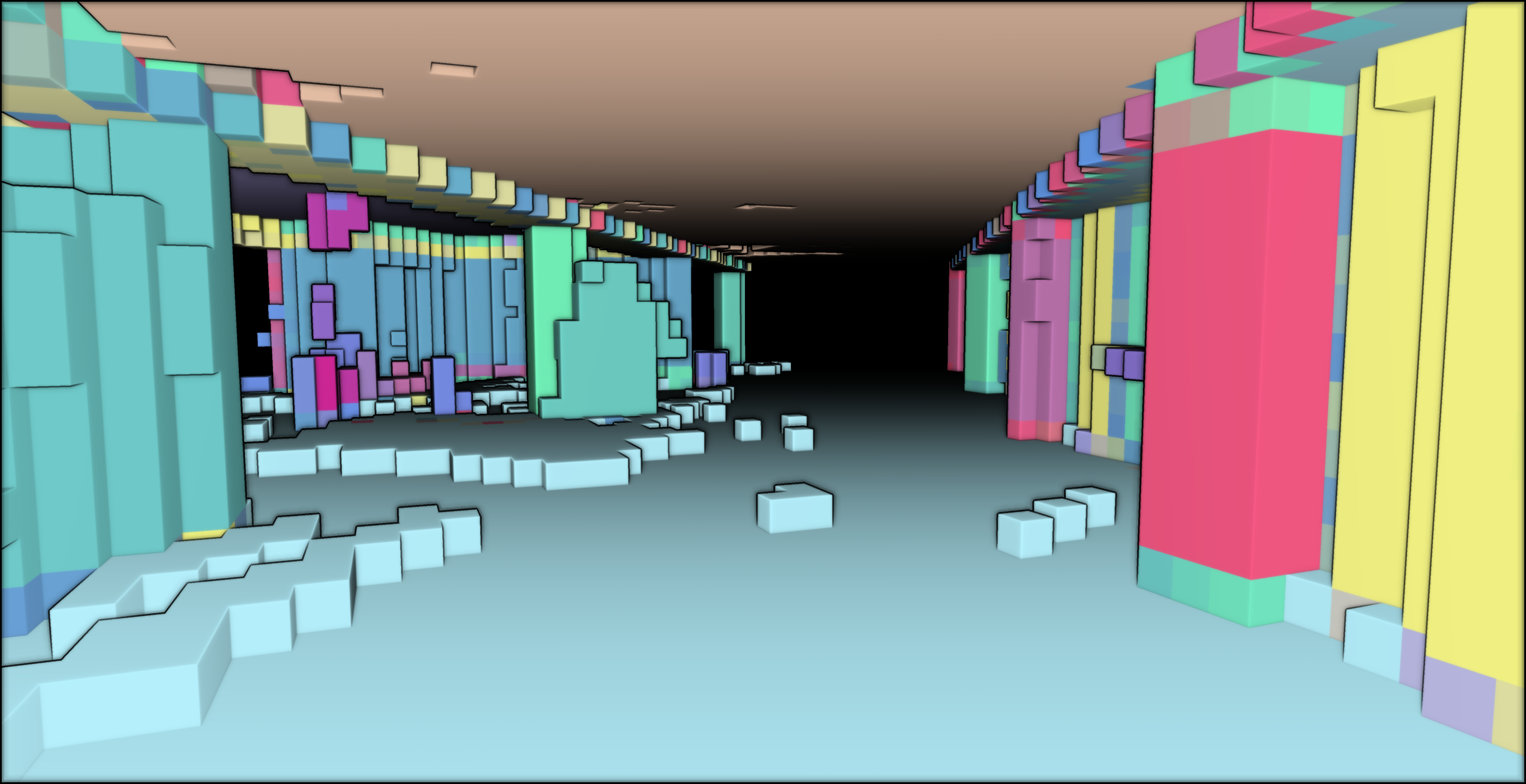
The final step is to visualize our result:o3d.visualization.draw_geometries([voxel_grid_clutter,voxel_grid_structural])

This is awesome! It looks like one of those computer games where the whole world is constructed out of cubes! And we can actually use the segment labels to guide our voxel modeling! This opens up many perspectives! But an issue remains. With Open3D, it is hard to extract the voxels that are not filled; So, having achieved the structuration of the voxelized point cloud, the subsequent step involves exploring voxel space modeling techniques to provide alternative perspectives for analyzing the spatial relationships and properties of the voxelized data, opening up new avenues for advanced point cloud modeling.

🤠 Ville: Voxelization is a different spatial representation of the same point cloud data. Great for robots if they need to avoid collisions! And for great for simulating… fire drills, for example!

9. Spatial Modelling based on 3D Shape Detection

In indoor modeling applications, the voxel-based representation of point clouds plays a pivotal role in capturing and analyzing the geometric properties of complex environments. As the scale and complexity of point cloud datasets increase, it becomes essential to delve deeper into voxel segmentation techniques to extract meaningful structures and facilitate higher-level analysis. Let us thus define a function that fits a voxel grid and return both filled and empty spaces:def fit_voxel_grid(point_cloud, voxel_size, min_b=False, max_b=False):
# This is where we write what we want our function to do.
return voxel_grid, indices

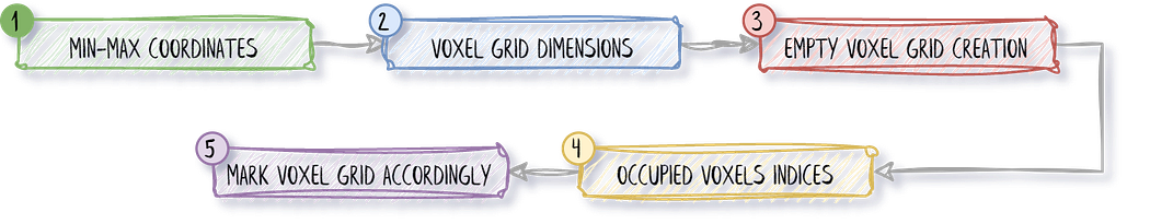
Within the function, we will (1) Determine the minimum and maximum coordinates of the point cloud, (2) Calculate the dimensions of the voxel grid, (3) Create an empty voxel grid, (4) Calculate the indices of the occupied voxels and (5) Mark occupied voxels as True.

This translates into the following code that we want to have inside this function:# Determine the minimum and maximum coordinates of the point cloud

if type(min_b) == bool or type(max_b) == bool:
min_coords = np.min(point_cloud, axis=0)
max_coords = np.max(point_cloud, axis=0)
else:
min_coords = min_b
max_coords = max_b
# Calculate the dimensions of the voxel grid
grid_dims = np.ceil((max_coords – min_coords) / voxel_size).astype(int)
# Create an empty voxel grid
voxel_grid = np.zeros(grid_dims, dtype=bool)
# Calculate the indices of the occupied voxels
indices = ((point_cloud – min_coords) / voxel_size).astype(int)
# Mark occupied voxels as True
voxel_grid[indices[:, 0], indices[:, 1], indices[:, 2]] = True

Our function is defined, and we can now use it to extract the voxels, segmented between structural, clutter, and empty ones:voxel_size = 0.3

#get the bounds of the original point cloud
min_bound = pcd.get_min_bound()
max_bound = pcd.get_max_bound()

ransac_voxels, idx_ransac = fit_voxel_grid(pcd_ransac.points, voxel_size, min_bound, max_bound)
rest_voxels, idx_rest = fit_voxel_grid(rest.points, voxel_size, min_bound, max_bound)

#Gather the filled voxels from RANSAC Segmentation
filled_ransac = np.transpose(np.nonzero(ransac_voxels))

#Gather the filled remaining voxels (not belonging to any segments)
filled_rest = np.transpose(np.nonzero(rest_voxels))

#Compute and gather the remaining empty voxels
total = pcd_ransac + rest
total_voxels, idx_total = fit_voxel_grid(total.points, voxel_size, min_bound, max_bound)
empty_indices = np.transpose(np.nonzero(~total_voxels))

🦚 Note: The nonzero() function from NumPy finds the indices of the nonzero elements in the ransac_voxels variable. The nonzero() function returns a tuple of arrays, where each array corresponds to the indices along a specific axis where the elements are nonzero. then we apply the np.transpose() NumPy function to the result obtained from np.nonzero(ransac_voxels). The transpose() function finally permutes the axes of the array. (effectively swapping the rows with the columns). By combining these operations, the code line transposes the indices of the nonzero elements of ransac_voxels, resulting in a transposed array where each row represents the coordinates or indices of a nonzero element in the original ransac_voxels array. 😊

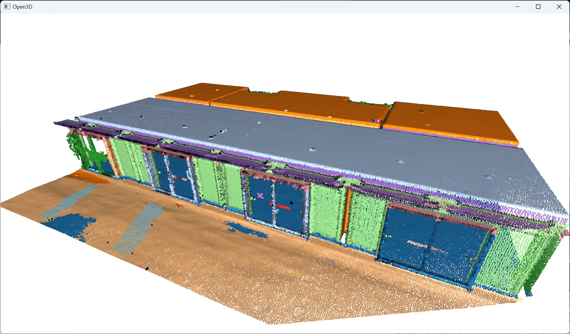
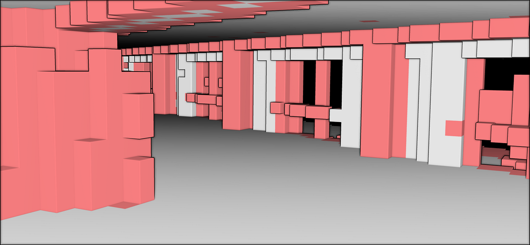
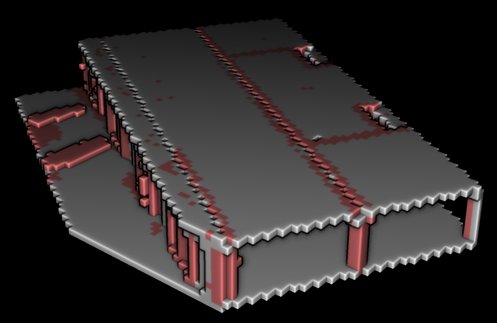
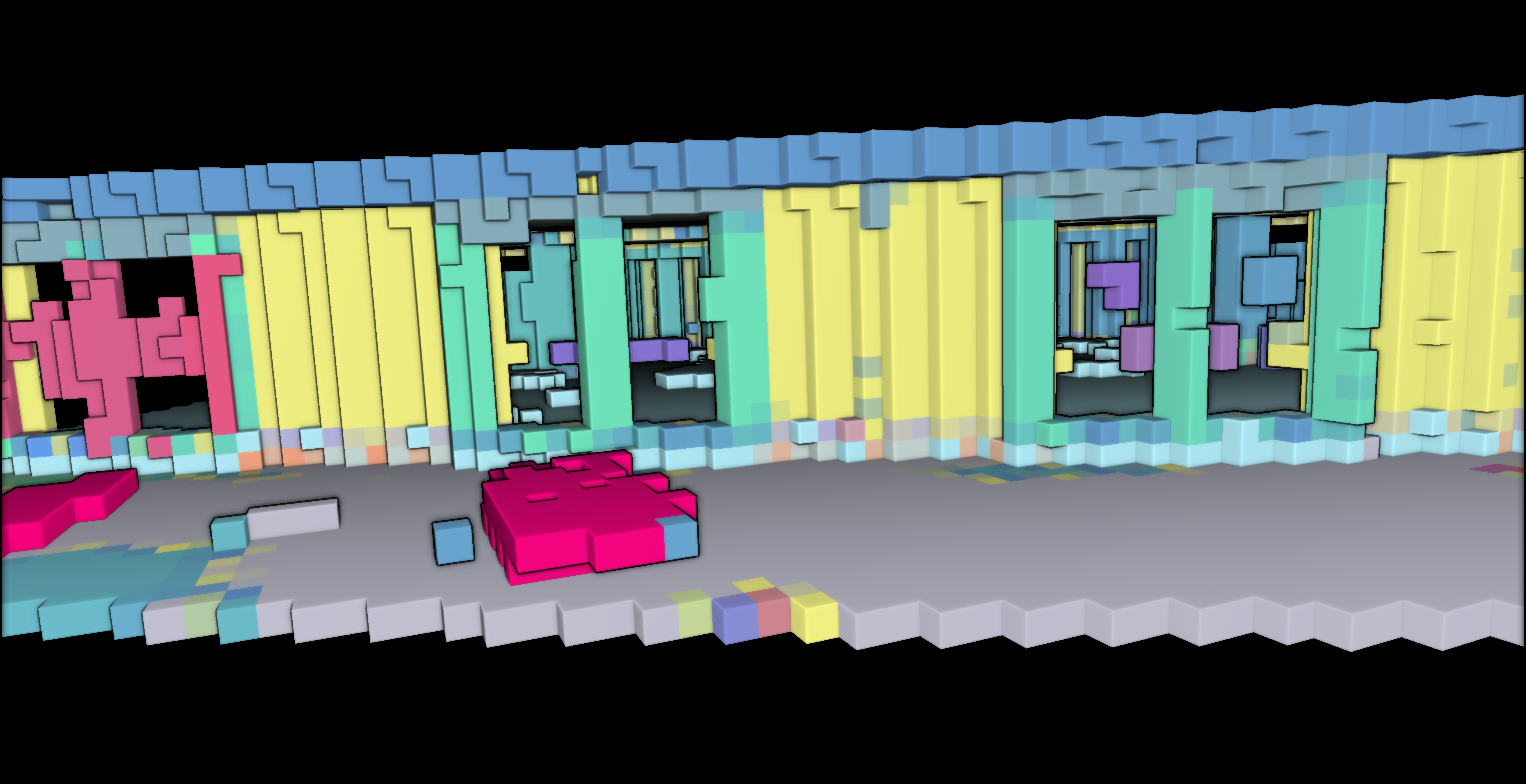
This voxel modeling approach offers valuable insights into the spatial relationships and properties of the voxelized data. To visualize the results as shown below outside of Python with transparency, we need to export our data.

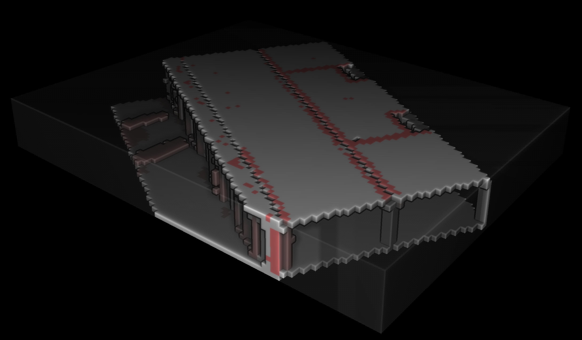
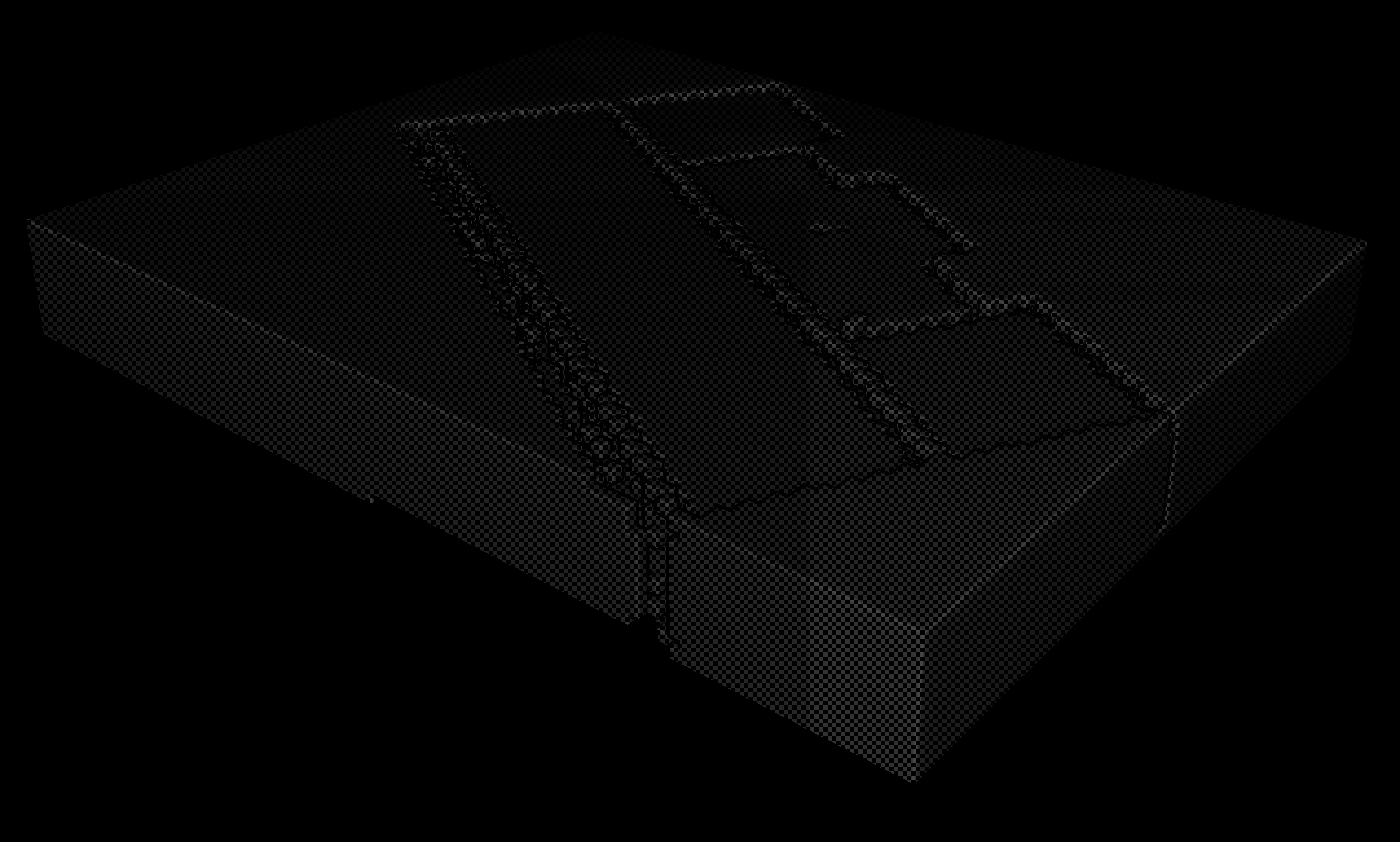
After achieving the structuration of the voxelized point cloud, the next step involves exporting both the point cloud and voxel data to external formats, facilitating interoperability and enabling seamless integration with other software tools and workflows. This export process ensures that the structured voxel data and the original point cloud can be easily shared, visualized, or utilized for further analysis in various applications, fostering a collaborative and versatile approach to point cloud data utilization.

10. Exporting 3D Datasets

Let us first focus on exporting the point cloud segmented datasets.

10.1. Segmented point cloud export

To export the segmented point cloud, we must ensure that we can write the label per point within a readable ASCII file. To do this, we will create a list of XYZ segments to which we will append the label feature. This can be done with the following for loop:xyz_segments=[]
for idx in segments:

print(idx,segments[idx])
a = np.asarray(segments[idx].points)
N = len(a)
b = idx*np.ones((N,3+1))
b[:,:-1] = a
xyz_segments.append(b)

From there, we want not to forget the remaining elements from the DBSCAN clustering, on which we apply the same principle:

rest_w_segments=np.hstack((np.asarray(rest.points),(labels+max_plane_idx).reshape(-1, 1)))

finally, we append this to the segments list:

xyz_segments.append(rest_w_segments)

all that we have to do is then to use numpy to export the dataset and visualize it externally:

np.savetxt(“../RESULTS/” + DATANAME.split(“.”)[0] + “.xyz”, np.concatenate(xyz_segments), delimiter=”;”, fmt=”%1.9f”)

Following the successful export of the segmented point cloud dataset, the focus now shifts to exporting the voxel dataset as a .obj file.

10.2. Voxel Model Export

To export the voxels, we first have to generate a cube for each voxel; These cubes are then combined in a voxel_assembly, stacked together to generate the final file. We create the voxel_modelling(filename, indices, voxel_size) function to do this:

def voxel_modelling(filename, indices, voxel_size):
voxel_assembly=[]
with open(filename, “a”) as f:
cpt = 0
for idx in indices:
voxel = cube(idx,voxel_size,cpt)
f.write(f”o {idx} \n”)
np.savetxt(f, voxel,fmt=’%s’)
cpt += 1
voxel_assembly.append(voxel)
return voxel_assembly

🦚 Note: the function cube() reads the provided indices, generates voxel cubes based on the indices and voxel size, writes the voxel cubes to a file, and keeps track of the assembled voxel cubes in the voxel_assembly list, which is ultimately returned by the function.

This is then used to export three different voxel assemblies:

vrsac = voxel_modelling(“../RESULTS/ransac_vox.obj”, filled_ransac, 1)
vrest = voxel_modelling(“../RESULTS/rest_vox.obj”, filled_rest, 1)
vempty = voxel_modelling(“../RESULTS/empty_vox.obj”, empty_indices, 1)

Conclusion

🦊 Florent: Massive congratulations 🎉! You just learned how to develop an automatic shape detection, clustering, voxelization, and indoor modeling program for 3D point clouds composed of millions of points with different strategies! Sincerely, well done! But the path certainly does not end here because you just unlocked a tremendous potential for intelligent processes that reason at a segment level!

🤠 Ville: So, now you’re wondering if we can make 3D modeling a completely hands-off process? We’re halfway there with the technique we’ve got. Why? Our technique can find parameters, for example, for the plane models. This is why the folks in academia call it parametric modeling. However, we still need to carefully choose some of the other parameters, such as the ones for RANSAC. I encourage you to experiment by applying your code on a different point cloud!

Going Further

The learning journey does not end here. Our lifelong search begins, and future steps will dive into deepening 3D Voxel work, exploring semantics, and point cloud analysis with deep learning techniques. We will unlock advanced 3D LiDAR analytical workflows. A lot to be excited about!

1. Lehtola, V., Nikoohemat, S., & Nüchter, A. (2020). Indoor 3D: Overview on scanning and reconstruction methods. Handbook of Big Geospatial Data, 55–97. https://doi.org/10.1007/978-3-030-55462-0_3
2. Poux, F., & Billen, R. (2019). Voxel-based 3D point cloud semantic segmentation: unsupervised geometric and relationship featuring vs deep learning methods. ISPRS International Journal of Geo-Information. 8(5), 213; https://doi.org/10.3390/ijgi8050213 — Jack Dangermond Award (Link to press coverage)
3. Bassier, M., Vergauwen, M., Poux, F., (2020). Point Cloud vs. Mesh Features for Building Interior Classification. Remote Sensing. 12, 2224. https://doi:10.3390/rs12142224

Learning Road to Expertise

If you want to get a tad more toward application-first or depth-first approaches, I curated on this website several learning tracks and courses to help you along your journey. Feel free to follow the ones that best suit your need, and do not hesitate to reach out directly to me if you have any questions or if I can give you some advice on your current challenges!

Open-Access Knowledge

• Medium Tutorials and Articles: Standalone Guides and Tutorials on 3D Data Processing (5′ to 45′)
• Research Papers and Articles: Research Papers published as part of my public R&D work.
• Email Course: Access a 7-day E-Mail Course to Start your 3D Journey
• Youtube Education: Not articles, not research papers, open videos to learn everything around 3D.

3D Online Courses

• 3D Python Crash Course (Complete Standalone). 3D Coding with Python.
• 3D Photogrammetry Course (Complete Standalone): Open-Source 3D Reconstruction.
• 3D Point Cloud Course (Complete Standalone): Pragmatic, Complete, and Commercial Point Cloud Workflows.
• 3D Object Detection Course (3D Python Recommended): Practical 3D Object Detection with 3D Python.
• 3D Collector’s Pack: Full Course Bundle + perks.

3D Learning Tracks

• 3D Segmentation Deck: From Classical 3D Segmentation to 3D Deep Learning and Unsupervised Applications
• 3D Collector’s Pack: Complete Course Track to address both 3D Applications and Code Layers.