This tutorial dives deep into the Marching Cubes algorithm, a powerful technique for meshing 3D point clouds using Python. We transform a point cloud into a 3D mesh, experiment with various parameters, and build a simple web app with a graphical user interface (GUI). This method bypasses the limitations of other reconstruction techniques like Poisson reconstruction, ball pivoting, and Delaunay triangulation.
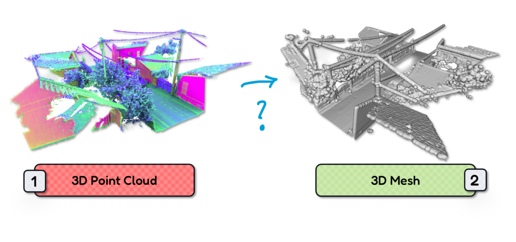
The world of 3D data is often a fragmented landscape. You have point clouds, rich in detail but lacking surface information. You have meshes, defining surfaces explicitly but often complex to create. Bridging this gap, converting point clouds to meshes, unlocks a wealth of possibilities, from realistic rendering and simulations to precise measurements and analysis.
Your mission, should you choose to accept it, is to master the art of mesh generation using the powerful Marching Cubes algorithm. We will navigate the intricacies of voxel grids, scalar fields, and iso surfaces, wielding the power of Python to transform raw point data into cohesive 3D models.
Mission Objective: 3D Mesh Reconstruction
Your primary objective is to develop a robust and efficient method for meshing point clouds. You will learn to control the meshing process through crucial parameters like voxel size and iso level, tailoring the output to your specific needs. Beyond mere conversion, you will strive for automation, empowering even non-programmers to effortlessly generate meshes through an intuitive web interface. Your secondary objective involves disseminating this knowledge, sharing your expertise with the wider 3D community.
🦊 Florent: The success of this mission depends on your understanding of the underlying principles. You must grasp the essence of the Marching Cubes algorithm, visualizing how it extracts a surface from a point cloud by cleverly analyzing a virtual grid. You must learn to wield the Python libraries like NumPy, Open3D, scikit-image, and SciPy, bending them to your will. Finally, you must embrace the power of Gradio, crafting a user-friendly interface to democratize access to this powerful technology.
Marching Cubes for 3D Mesh: Foreword
The world of 3D digital representation revolves around two fundamental data structures: point clouds and meshes. Understanding their nuances is crucial for anyone working with 3D data, especially when aiming to convert between these formats.
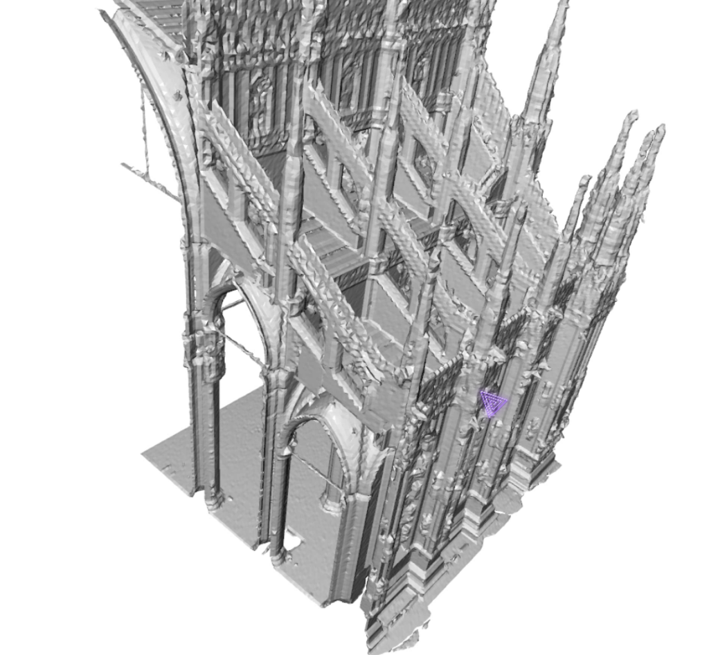
This enhanced tutorial delves deeper into the concepts of point clouds and meshes explains the intricacies of the Marching Cubes algorithm and provides a detailed Python implementation for converting point clouds to meshes. We’ll explore this powerful technique’s why, how, and practical implications, empowering you to effectively manipulate and visualize 3D data.
🗝️ Key Takeaways
- Point clouds represent 3D shapes as collections of points with spatial coordinates and optional attributes.
- Meshes represent 3D shapes as connected triangles, defining surfaces explicitly.
- The Marching Cubes algorithm bridges the gap, creating meshes from point clouds using an implicit surface representation.
- Understanding parameter tuning and automation is crucial for optimal mesh generation.
- Building a web app democratizes access to this technology.
Introduction to Point Clouds and 3D Meshes
Imagine capturing an object’s 3D shape. One approach involves scanning its surface with a laser scanner, which generates a point cloud.
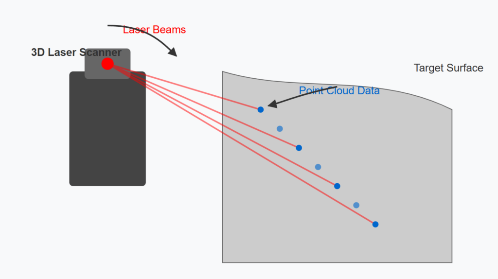
This point cloud is a collection of millions or even billions of individual points.
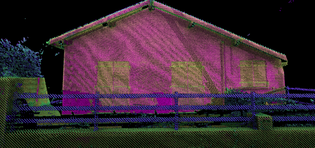
Each point holds its spatial coordinates (x, y, z) and potentially other attributes like color, intensity, or classification labels. Point clouds are raw and direct representations of 3D shapes, preserving fine details but lacking explicit surface information.
Alternatively, you can represent the object’s shape as a mesh. A mesh constructs the surface using interconnected triangles. Each triangle is defined by three vertices, and their connections form a network that approximates the object’s surface.
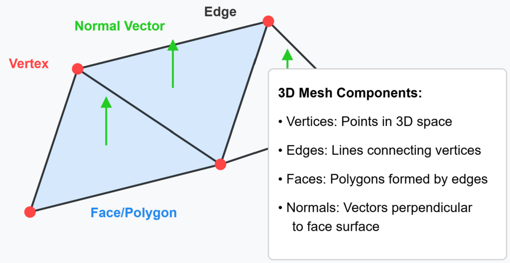
Meshes explicitly define the surface, enabling calculations like surface area and volume and facilitating rendering with realistic lighting and shading. However, creating meshes directly can be complex and often relies on algorithms that infer surface connections from point clouds.
What we want to do, is bridging the gap between these two representations through the Marching Cubes algorithm. It a is bridgellows us to create a mesh from a point cloud by implicitly defining a surface. Instead of directly connecting points, the algorithm creates a virtual surface around the point cloud and then “extracts” a mesh from this surface.
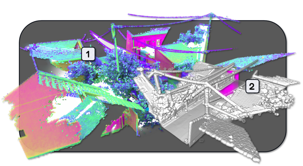
Deep Dive into the Marching Cubes Algorithm for 3D Mesh
The Marching Cubes algorithm, developed by Lorensen and Cline in 1987, is a clever technique for creating a mesh from a volumetric dataset. Think of the point cloud as being embedded within a virtual grid, similar to a 3D chessboard. Each cell in this grid, called a voxel, is examined by the algorithm.
The algorithm works by imagining an implicit surface flowing through this grid. This surface isn’t defined directly but is implied by the values of a scalar field at the corners of each voxel. In our case, the scalar field represents the distance from each grid point (voxel corner) to the nearest point in the input point cloud.
The crucial concept here is the iso level or iso surface. Imagine contour lines on a topographic map. Each contour line connects points of equal elevation.
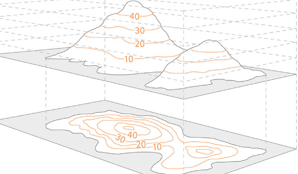
The iso surface in Marching Cubes works similarly but in 3D. It connects points in the grid where the scalar field has the same value. This iso surface represents the “boundary” of our mesh.
For each voxel, the algorithm checks the values of the scalar field at its eight corners. If a corner’s value is above the iso level, it’s considered “outside” the surface; if below, it’s “inside.” Based on the combination of “inside” and “outside” corners, the algorithm determines how the iso surface intersects the voxel. This intersection is then represented by one or more triangles, forming a piece of the final mesh.
By repeating this process for every voxel in the grid, the algorithm creates a complete mesh that approximates the surface defined by the point cloud.
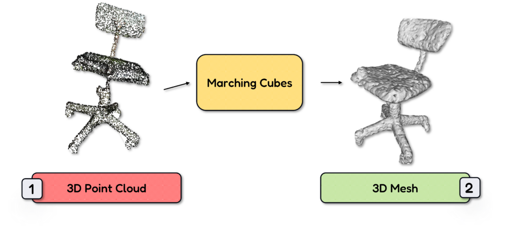
The choice of iso level is critical. A low iso level generates a tight mesh, closely following the point cloud, potentially capturing noise and fine details. A high iso level creates a smoother, more generalized mesh.
🦚 Note: The iso_level_percentile parameter in our Python implementation controls this level, expressed as a percentile of the distances computed in the scalar field. The size of the voxels, determined by voxel_size, also affects the result. Smaller voxels yield finer meshes, capable of capturing more details but requiring more computation. Larger voxels create coarser meshes, faster to compute but potentially missing subtle features.
Step 1: 3D Python Setup
Let us make sure you have everything that is needed to start working.
Libraries Import
This stage involves importing the necessary Python libraries: NumPy for numerical operations, Open3D for point cloud and mesh handling, scikit-image for the Marching Cubes implementation, and SciPy for spatial data structures and computations.
import numpy as np
import open3d as o3d
from skimage import measure
from scipy.spatial import cKDTree
Gathering 3D Point Clouds
Here, you collect the point cloud data you want to process. This might involve reading files from disk (e.g., .ply, .las, .xyz formats) or acquiring data from other sources. Each point cloud is typically represented as a data structure containing the x, y, and z coordinates of each point, along with any additional attributes like color or intensity.
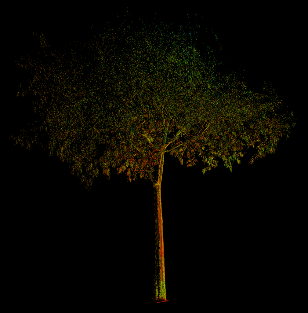
🦚 Note: To start things off, I recomment that you use a small point cloud to test out the parameters of the approach.
3D Python Libraries, Software, Tools and Resources
Below, I listed all the various Tools and libraries that we are going to leverage in this tutorial.
- Anaconda: https://www.anaconda.com/ – A popular Python distribution platform for data science and machine learning, providing package management and environment control.
- Python Libraries: These can be installed via pip (package installer for Python) within your Anaconda environment or any other Python environment.
- NumPy: https://numpy.org/ – Fundamental library for numerical computing in Python, providing powerful array operations.
- Open3D: http://www.open3d.org/ – Library specifically designed for 3D data processing, including point cloud and mesh manipulation, visualization, and algorithms.
- scikit-image: https://scikit-image.org/ – Image processing library built on top of NumPy, providing tools for image analysis, segmentation, and more (including the Marching Cubes implementation).
- SciPy: https://scipy.org/ – Library built on NumPy, providing advanced scientific computing capabilities, including spatial data structures like KD-Trees.
- Gradio: https://gradio.app/ – Python library for creating user interfaces for machine learning models, allowing you to build interactive web demos.
- Software:
- CloudCompare: https://www.danielgm.net/cc/ – Open-source 3D point cloud and mesh processing software, useful for visualizing, analyzing, and editing 3D data. It also has a command-line interface for batch processing.
Step 2: The Marching Cubes 3D Meshing Function
This is the core of the process, where the magic of Marching Cubes happens. Let me detail the core components of the point cloud to 3D mesh strategy, as illustrated below.

The Marching Cubes: 3D Mesh Python Function Definition
First off, let us define our two parameters that are going to be used in our function:
voxel_size=0.1
iso_level_percentile=20
Great, I will not create more traciton there, but let me detail all the seven steps that happens within the 3D Meshin, Marching Cubes Function:
a. Open3D to PCD
We load our point cloud with Open3D, and then we can put that as a numpy array. This ensures compatibility with downwards processes.
pcd = o3d.io.read_point_cloud(dataset)

# Convert Open3D point cloud to numpy array
points = np.asarray(pcd.points)
b. Bounds Computation
Let us determine the minimum and maximum extents of the point cloud along each axis (x, y, z). This defines the bounding box that will enclose our voxel grid.
# Compute the bounds of the point cloud
mins = np.min(points, axis=0)
maxs = np.max(points, axis=0)
c. Creating a 3D Grid for the 3D Point Cloud
Let us create a regular 3D grid, or voxel grid, within the bounding box. The voxel_size parameter determines the spacing between grid points; each cell in this grid is a voxel.
# Create a 3D grid
x = np.arange(mins[0], maxs[0], voxel_size)
y = np.arange(mins[1], maxs[1], voxel_size)
z = np.arange(mins[2], maxs[2], voxel_size)
x, y, z = np.meshgrid(x, y, z, indexing='ij')
d. KD-Tree for Efficiency
It is time to construct a KD-Tree (k-dimensional tree) from the point cloud data. Shortly, KD-Trees are efficient spatial data structures that facilitate fast nearest-neighbor searches. But at this stage you should have that in mind 😉
# Create a KD-tree for efficient nearest neighbor search
tree = cKDTree(points)
e. Scalar Field: Distance to Nearest Point
For each grid point (corner of a voxel), we are going to calculate the distance to the nearest point in the point cloud using the KD-Tree. This distance value becomes the scalar field value at that grid point, as shown below:
# Compute the scalar field (distance to nearest point)
grid_points = np.vstack([x.ravel(), y.ravel(), z.ravel()]).T
distances, _ = tree.query(grid_points)
scalar_field = distances.reshape(x.shape)
f. Determine the Iso Level
All right, it is time to focus on the ISO level. The ISO level defines the surface threshold for the Marching Cubes algorithm. It’s calculated as a percentile of the distances computed in the previous step. The iso_level_percentile parameter controls this, and I illustrate it below.
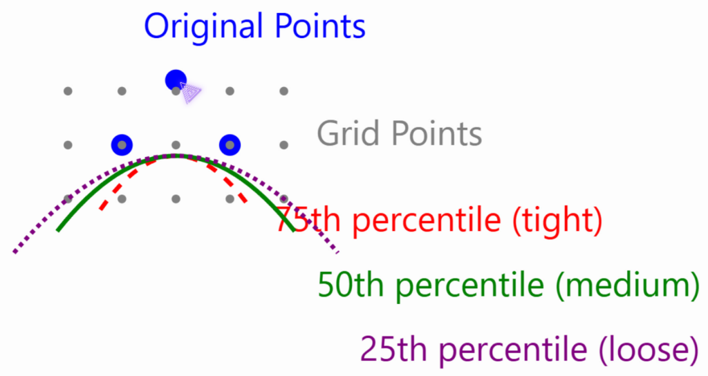
# Determine iso-level based on percentile of distances
iso_level = np.percentile(distances, iso_level_percentile)
g. Apply Marching Cubes
We are almost there: we can now call our marching cube function. The skimage.measure.marching_cubes function takes the scalar field and iso level as input.
# Apply Marching Cubes
verts, faces, _, _ = measure.marching_cubes(scalar_field, level=iso_level)
This function analyzes each voxel and generates triangles based on how the iso surface intersects the voxel. We are finally ready to go onto 3D Mesh Post-Processing.
Step 3. 3D Mesh Post-Processing
At this stage, our mesh is almost ready. We just wantto put him back in its original position, and generate the 3D mesh object. Let us firs address the 3D Transformations.
Scale and Translate
The vertices of the generated triangles are initially in voxel grid coordinates. This step scales and translates the vertices back to the original point cloud coordinate system. We can move as illustrated below.
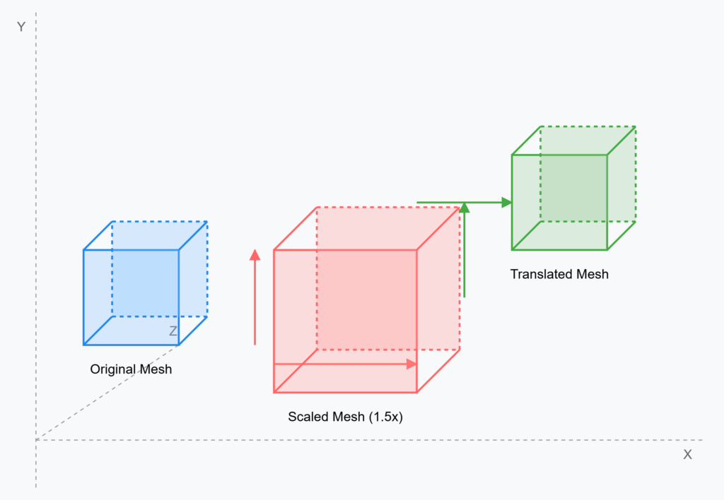
which means with python code:
# Scale and translate vertices back to original coordinate system
verts = verts * voxel_size + mins
Beautiful! Now, we can generate our 3D Mesh from our point cloud.
Creating our 3D Mesh
Let us create an Open3D TriangleMesh object with its scaled and translated vertices and triangle connectivity information (faces). We can use Open3D to do just that, as shown below.
# Create mesh
mesh = o3d.geometry.TriangleMesh()
mesh.vertices = o3d.utility.Vector3dVector(verts)
mesh.triangles = o3d.utility.Vector3iVector(faces)
From there, we can leverage an additionnal step: Normals Computation.additional
Computing 3D Mesh Normals
To populate the 3D mesh with normals, let us compute Vertex normals. These normals are crucial for proper lighting and shading during rendering, making the mesh appear smooth.
# Compute vertex normals
mesh.compute_vertex_normals()
Beautiful! At this stage, we are ready to move onto visualizing our 3D Mesh.
🦚 Note: The full process depends on the two defined parameters, the voxel size and iso percentile choice. The first parameter, the voxel size, will highly influence the computing time, especially for big point clouds. The second will also affect the computing time but as a lower impact. however, its geometric impact is significant.
Step 4. 3D Mesh Visualization
The moment you have been waiting for is there: we can now visualize our 3D Mesh, with the following command:
# Visualize the result
o3d.visualization.draw_geometries([mesh], mesh_show_back_face=True)
This results in the following.
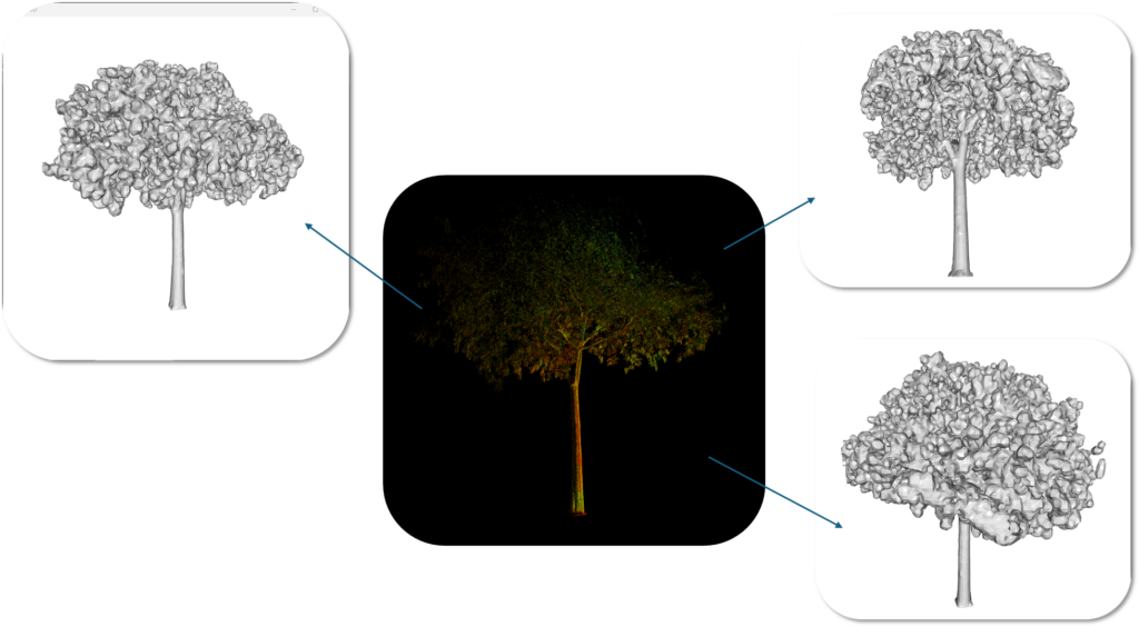
Displaying the generated mesh using Open3D’s visualization functions allows us to inspect the results. As you can see, the 3D Tree Mesh is very interestingly well meshed.
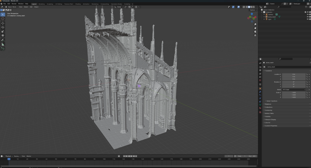
🦚 Note: You can save the mesh to a file (e.g., .ply, .obj, .stl) for use in other applications, such as Blender
Step 5. Auto Parameters Estimation (Marching Cubes)
To automate the meshing process, you can estimate suitable values for voxel_size and iso_level_percentile. This is especially useful for very large point clouds, consider optimizing computations. Techniques like chunking (processing the point cloud in smaller blocks), parallelization, and efficient data structures can significantly improve performance.
🦚 Note: These techniques are taught in the 3D Segmentor OS, which you can find below.
As a way to guide you on this path, I recommend first to estimate the voxel size. You can use the average distance to k-nearest neighbors in the point cloud, and use this value to guide the voxel size definition with some kind of heuristics. Then, to Estimate Iso Level Percentile, you can use the distribution of distances from the scalar field to determine a suitable percentile. This means computing a Coefficient of Variation (CV) from the distances (standard deviation divided by the mean).
Finally, you can Adjust the percentage based on your CV. Higher CV values (more spread-out points) generally lead to lower percentiles, and vice-versa.
Step 6. Creating a web-app with Gradio
Let us build a user-friendly web interface using Gradio. This interface can allow users to upload point cloud files, adjust parameters (voxel size, iso level), and visualize the generated meshes directly in their browser. This democratizes access to the meshing process, making it accessible even to non-programmers.
To use Gradio to build a simple GUI, we usually follow such a pattern:
import gradio as gr

with gr.Blocks() as app:
    # ... (Gradio interface setup as described in the audio)
This creates a drag-and-drop interface to upload a point cloud and generate the mesh directly in the browser.
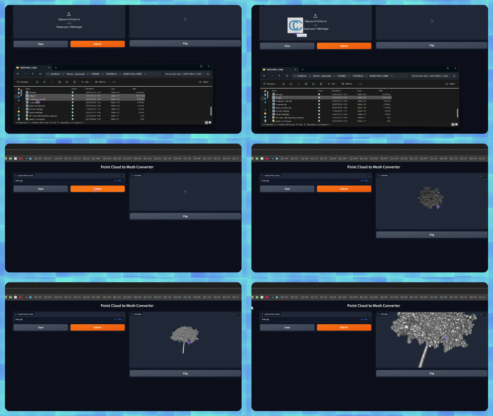
To get the 3D Model View, you can use the code below:
# Create Gradio interface
iface = gr.Interface(
    fn=point_cloud_to_mesh,
    inputs=gr.File(
        label="Upload Point Cloud",
        file_types=[".pcd", ".ply", ".xyz", ".pts"],
    ),
    outputs=gr.Model3D(
        clear_color=[0.0, 0.0, 0.0, 0.0],  label="3D Model"),
    title="Point Cloud to Mesh Converter",
    examples=[],
    cache_examples=False,
    )

# Launch the interface
if __name__ == "__main__":
    iface.launch()
This code creates a web-based user interface using Gradio, designed to convert point cloud files into 3D meshes. The interface is configured with a file upload component that specifically accepts point cloud files (in .pcd, .ply, .xyz, or .pts formats) and displays them in a 3D model viewer with a transparent background. The processing is handled by the function called point_cloud_to_mesh which contain the actual conversion logic that we explained before.
When the script is run directly, it launches a web page titled “Point Cloud to Mesh Converter” where users can simply upload their point cloud files and view the resulting 3D mesh in an interactive viewer. The interface is streamlined with no example files and disabled caching, focusing on providing a straightforward conversion service.
Conclusion
This tutorial has explored the foundational concepts of point clouds and meshes, provided a comprehensive explanation of the Marching Cubes algorithm, and demonstrated its practical application using Python. By understanding the interplay of parameters like voxel_size and iso_level_percentile, you can fine-tune the mesh generation process to achieve desired levels of detail and smoothness. Building a Gradio web app democratizes access to this technology, enabling users without programming expertise to interact with and visualize 3D data effectively.
This workflow empowers you to bridge the gap between point clouds and meshes, opening doors to a wide range of applications in various fields. For delving deeper into point cloud processing, mesh optimization, and related topics, consider exploring resources and other Open Tutorials below.
3D Tutorials (Open-Access)
- 3D Point Cloud Labeling from Photos with Python (and why AI can’t design it for you)
- 3D Pipeline Architecture: A Founder’s Blueprint
- Multi-View Engine for 3D Generative AI Models (Python Tutorial)
- 3D Scene Graphs for Spatial AI with NetworkX and OpenUSD
- 3D Reconstruction Pipeline: Photo to Model Workflow Guide
- Synthetic Point Cloud Generation of Rooms: Complete 3D Python Tutorial
- 3D Generative AI: 11 Tools (Cloud) for 3D Model Generation
- 3D Gaussian Splatting: Hands-on Course for Beginners
- Building a 3D Object Recognition Algorithm: A Step-by-Step Guide
- 3D Sensors Guide: Active vs. Passive Capture
- 3D Mesh from Point Cloud: Python with Marching Cubes Tutorial
- How To Generate GIFs from 3D Data with Python
- 3D Reconstruction from a Single Image: Tutorial
- 3D Reconstruction Methods, Hardware and Tools for 3D Data Processing
- 3D Deep Learning Essentials: Ressources, Roadmaps and Systems
🐦 In Brief: This tutorial demonstrates a comprehensive workflow for meshing point clouds with the Marching Cubes algorithm. The approach is flexible, allows for parameter tuning and automation, and culminates in a user-friendly web app. This method provides a robust and accessible way to generate 3D meshes from point cloud data. For further optimization and advanced techniques, consider the 3D Segmentor OS track.
