Python Guide for Euclidean Clustering of 3D Point Clouds

Python Tutorial for Euclidean Clustering of 3D Point Clouds with Graph Theory. Fundamental concepts and sequential workflow for unsupervised segmentation.

As you are developing the next generation of AI systems, you face a critical bottleneck: efficiently segmenting 3D point clouds to extract meaningful objects.

This process is often manual, time-consuming, and prone to errors, especially when dealing with the massive datasets required for cutting-edge applications. Imagine spending days meticulously labeling individual chairs, tables, and lamps in a single room’s point cloud – now multiply that effort by the thousands of rooms your AI needs to understand. This is simply not scalable for real-world deployment.

The consequences of inefficient segmentation are significant. It directly impacts your project deadlines, limits the scope of your AI’s capabilities, and ultimately hinders progress in your field.

We need a solution that automates this process while ensuring accuracy and scalability.

Why do we use Graph Theory for Euclidean Clustering?

Aside from sounding cool, why do I take three weeks off to write a Python tutorial on graph theory for 3D data?

The short answer is that it is extremely useful for understanding 3D scenes. It can transform how efficiently you process 3D datasets for decision-making scenarios.

But there are many challenges to be aware of. 

If we take a step back, our eyes can capture spatial information and then process it through our cognition system. And this is where the magic lies: our brain helps us make sense of the scene and its relational decomposition.

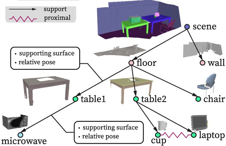
With internal knowledge representation, you can instantly know that your scene is made of floors and walls, that the floor hosts chairs and tables, and that, in turn, the cup, microwave, and laptop stand on the desks.

Mimicking this with 3D Tech means we need to find a way to leverage a 3D dataset that represents the scene and then build a decomposition into the main constituents: A clustering.

From my example, you can understand how “connectivity” plays a major role: it is simple to distinguish “objects” that do not touch (once the support is removed, i.e., the ground). But can we achieve this decomposition efficiently with 3D digital datasets?

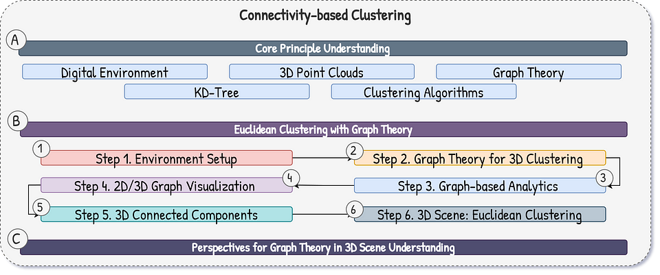
Let us develop an advanced solution with Graph Theory for 3D datasets that builds on the workflow illustrated below.

Now, let me give you the mission brief.

🦊 Florent Poux, Ph.D. : If you are new to my (3D) writing world, welcome! We are going on an exciting adventure that will allow you to master an essential 3D Python skill. Before diving, I like to establish a clear scenario, the mission brief.

Once the scene is laid out, we embark on the Python journey. Everything is given. You will see Tips (🦚Notes and 🌱Growing) to help you get the most out of this article.

The 3D Data Mission Brief

You are organizing a massive library of 3D objects to develop the next-generation AI system that can identify in real-time the model of each piece of furniture. The issue: You have three days to do ten entire buildings.

You load your 3D point clouds and try the first approach: manual segmentation. You can quickly see that it becomes a significant bottleneck for identifying individual objects like chairs, tables, and lamps in a scanned environment.

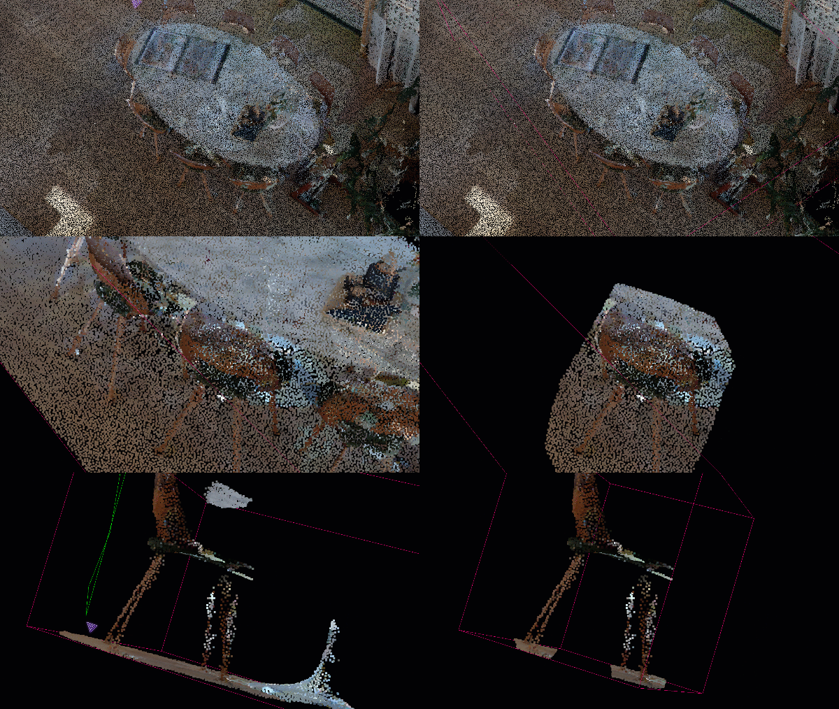
You encounter memory limitations and juggle multiple software platforms, each introducing its own constraints, learning curves, and errors.

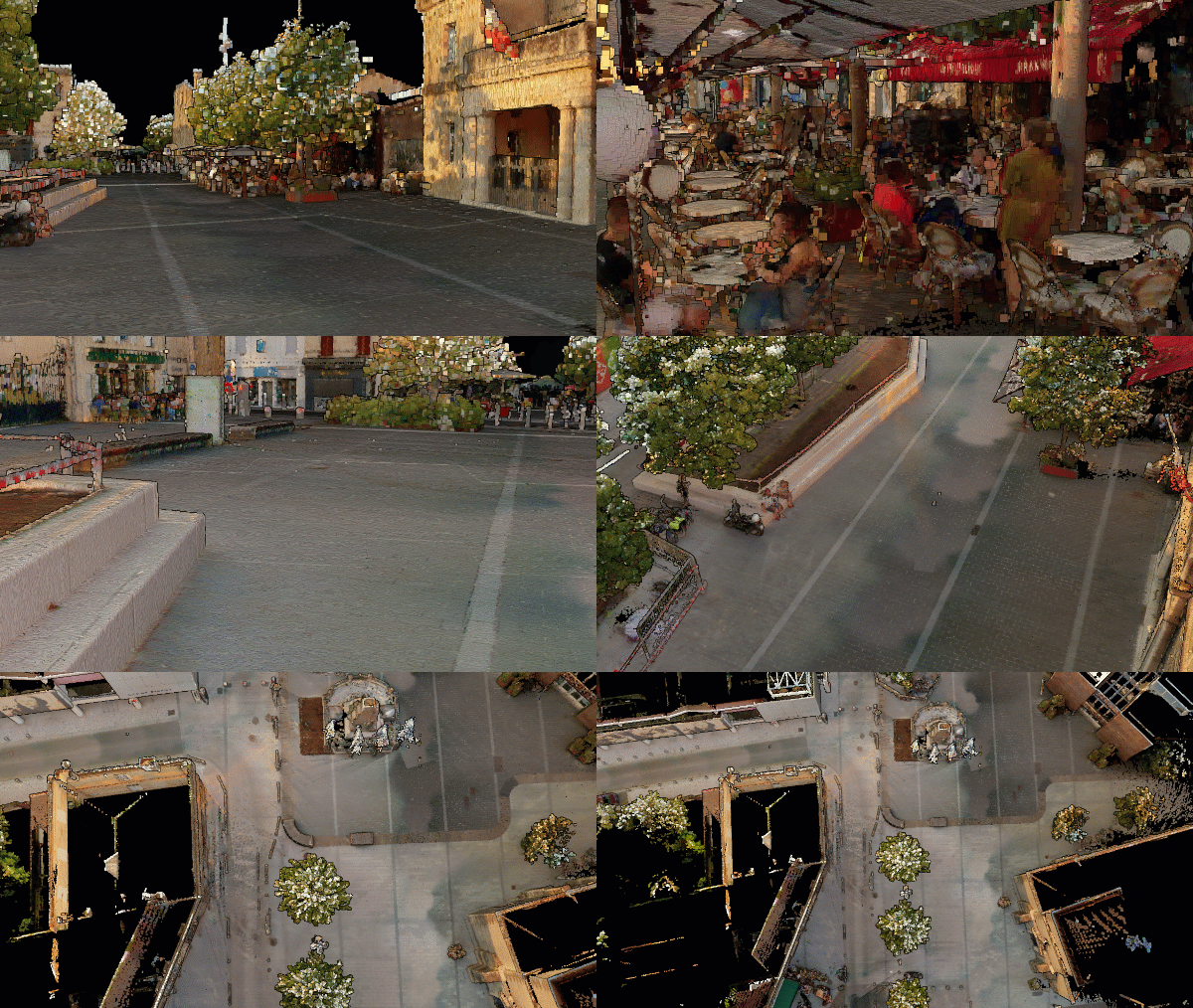
After losing one day in a tedious cycle of exporting, importing, and converting data across various tools, you feel discouraged by your disjointed workflow, which hampers productivity and scalability.

You decide to get a good night of sleep, and while dreaming, you imagine a streamlined solution that harnesses the power of graph theory to redefine how you approach point cloud segmentation.

The Revelation: Euclidean Clustering

The little dreambee tells you to automate the process by employing Euclidean clustering in Python, eliminating the reliance on manual intervention. 

This innovative method organizes point clouds into structured graphs, where each point is a node connected by edges that signify proximity. Then, through algorithms for connected component analysis, you could enable efficient, automated delineation of objects, transforming how you analyze and interpret the 3D data.

You wake up, and that is it: You are going to develop a solution that presents a clear and effective method: Euclidean clustering utilizing graph theory in Python. 

Initially, you eliminate significant structural components such as walls and floors, which can be segmented using alternative methods like RANSAC, thereby isolating the objects of interest.

Subsequently, you want to create a graph in which each point is represented as a node, and connections. This graphical representation and effective algorithms should then be able to leverage connected component analysis to enable the automatic delineation of individual objects, which is significantly more efficient than manual segmentation.

It is time to dive into the solution! But first, here are some words on the core principles of what we are going to use.

Euclidean Clustering: Core Principle

For wielding Connectivity-based clustering, it is important to understand our digital environments, the role of point clouds, graph theory, KD-Trees, and Clustering algorithms (see below)

Aside from digital environments, let me highlight the core concepts that we leverage and the related resources if you feel like you need a refresher:

1. 3D Point Cloud (Unstructured Data): A point cloud represents a 3D scene as a collection of individual points, each with its own 3D coordinates. Unlike mesh data, which explicitly defines surface connectivity, point cloud data is unstructured. This lack of inherent relationships between points poses a challenge for segmentation.
2. Graph Theory Basics: Graph theory provides a powerful framework for representing relationships between entities. A graph consists of nodes (vertices) connected by edges. In our case, each point in the point cloud becomes a node. Edges connect spatially proximate points, transforming the unstructured point cloud into a structured graph.
3. KD-Tree: A KD-Tree (K-Dimensional Tree) is a space-partitioning data structure that efficiently organizes points in a K-dimensional space (3D in our case). It recursively divides the space with hyperplanes, creating a tree-like structure. This initially enables fast nearest-neighbor searches, which is crucial for efficiently finding points within a given radius.
4. (3D) Clustering: Our approach centers on clustering, which transforms disconnected points into meaningful groups representing objects or distinct regions within the 3D scene. While other approaches like K-Means or DBSCAN exist, we unveil graph-based clustering to leverage connectivity. Our method relies on constructing a graph from the point cloud and then identifying connected components within this graph. Each connected component represents a cluster.

We can now proceed with a comprehensive Python implementation.

The Graph-based Clustering Python Workflow

Let me illustrate the 6-step workflow below using both a synthetic dataset for demonstration and a real-world point cloud to highlight its practical application.

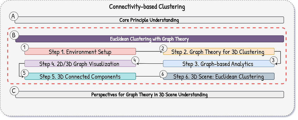
The solution is designed to provide an effective tool for managing point cloud data and maximizing its potential for unsupervised segmentation scenarios.

Step 1. Environment Setup for Euclidean Clustering

The first stage is to set our environment for a successful project. We have three main constituents: the Python setup, the data setup, and the utilities.

Python Setup

Concerning our Python setup, we leverage Python 3.10 with Anaconda. After the creation of a virtual environment using Anaconda, we install the five following libraries:

• NumPy for numerical operations: https://numpy.org/
• SciPy for scientific computing, including KD-Tree implementation: https://scipy.org/
• NetworkX for graph manipulation and analysis: https://networkx.org/
• Matplotlib for visualization and color mapping: https://matplotlib.org/
• Open3D for advanced 3D data processing and visualization

To install these libraries, we use the pip package manager as follows:

pip install numpy scipy networkx matplotlib open3d

🦚 Note: If you want to ensure you understand how to set up your environment for local 3D development quickly, I encourage you to follow up this video tutorial. You may want to use an IDE for easier development; I use Spyder, installed with pip install spyder, and launched with spyder.

3D Data Setup

Then, we gather a 3D point cloud of an indoor scene that our method is going to attack (see the image below):

The dataset was obtained using the Naavis VLX2 hand-held laser scanner.

Utilities

Finally, we are going to leverage CloudCompare as a supplementary tool for visualization and demonstration outside of the Python environment.

Now that we are set, let us test our system by loading our point cloud (e.g., in PLY format, given in my Drive folder) into Python:

# Importing the libraries
import numpy as np
from scipy.spatial import KDTree
import networkx as nx
import matplotlib.pyplot as plt
import open3d as o3d

# Load point cloud (PLY format)
pcd = o3d.io.read_point_cloud("../DATA/room_furnitures.ply")
translation = pcd.get_min_bound()
pcd.translate(-translation)

# Visualization with Open3d
o3d.visualization.draw_geometries([pcd])

We leverage Open3D (o3d) to load a point cloud dataset representing our room with furniture, as illustrated below. 

As you can see, we got rid of the walls and the floor, by using RANSAC algorithm for planar shape detection

3D Model Fitting for Point Clouds with RANSAC and Python
A 5-Step Guide to create, detect, and fit linear models for unsupervised 3D Point Cloud binary segmentation: RANSAC…towardsdatascience.com

The critical operation here is translating the point cloud to its minimum bound, effectively centering the dataset at the origin. This preprocessing step is crucial for subsequent geometric operations, ensuring that our spatial analysis starts from a standardized reference point. By calling pcd.translate(-translation), we shift the entire point cloud, which helps in maintaining consistent spatial relationships during further processing.

🦚 Note: The visualization using o3d.visualization.draw_geometries([pcd]) allows us to inspect the loaded point cloud visually, providing an immediate verification of data integrity and spatial configuration. This step is fundamental in 3D data science, as visual confirmation helps us quickly identify potential issues or characteristics in the dataset before diving into complex analytical procedures.

Great, we can move on to the second stage: constructing our graph.

Step 2. Graph Theory for 3D Euclidean Clustering

Let us generate graphs with Python. But before moving there, I want to give you the fundamentals of the Graph Theory that we are going to leverage, so that what I code make sense.

Graph Theory Fundamentals for 3D Data

Let’s explore the fundamental concepts of graph theory used in our point cloud clustering approach, drawing directly from the interactive explanation presented in the audio tutorial. Visualizing these concepts makes them much more intuitive and engaging.

What is a Graph?

A graph is a structure composed of vertices (also called nodes) and edges.

Think of vertices as individual entities and edges as connections or relationships between these entities. The graph above is composed of six vertices, and 7 edges, that we denote as such:

The vertices (nodes) holds information relevant to the entity it represents. In our point cloud scenario, each point’s 3D coordinates would be associated with a vertex. The Edges (Connections) are represented as lines connecting vertices. They signify a relationship between the entities represented by the vertices. In our case, an edge between two vertices would indicate that the corresponding points in the point cloud are spatially close to each other, within the defined radius.

Graph Properties

Now, you have some Key Graph Properties to be aware of:

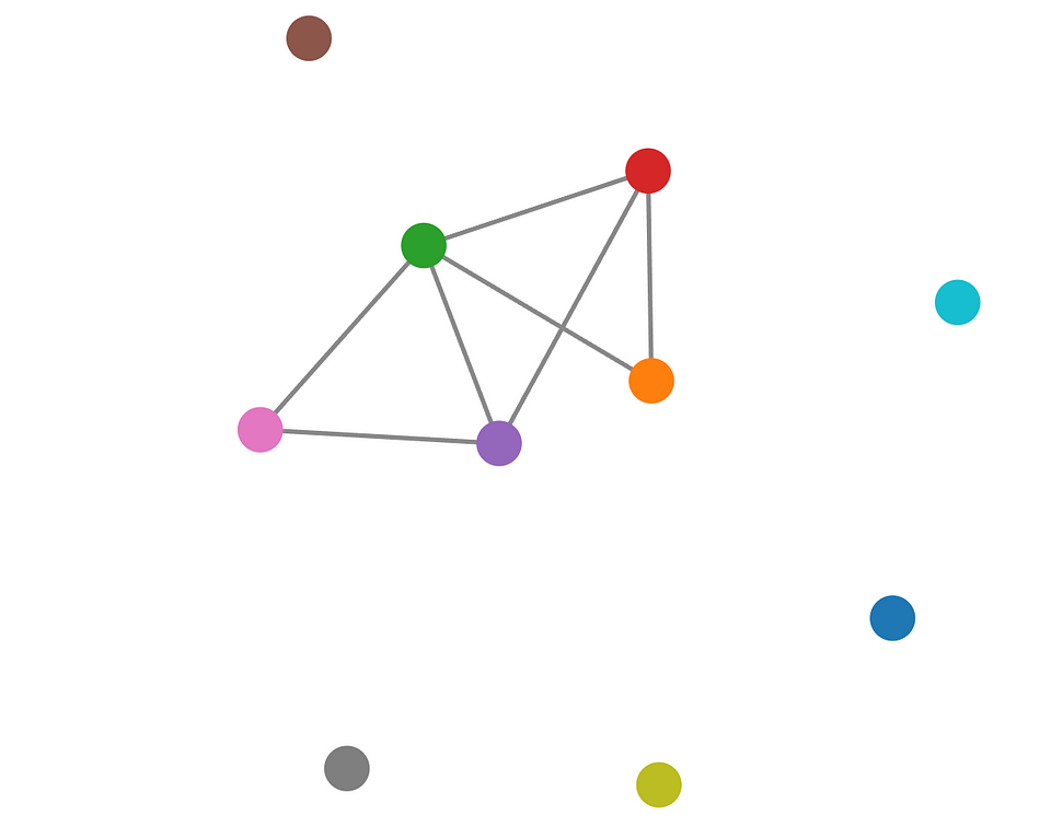
First, the order of a graph is simply the number of vertices it contains. In the example, you have 10 vertices, hence the order is 10. Adding or removing vertices changes the order of the graph. In our point cloud graph, the order is equal to the number of points in the cloud.

Then, the size of a graph refers to the number of edges (in the example above, this is 7). As we connect or disconnect vertices, the size of the graph changes accordingly. In our point cloud graph, the size reflects the density of connections based on the chosen radius and the max_neighbors parameter.

Finally, the degree of a vertex is the number of edges connected to it (see illustration below). 

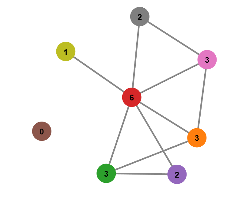
A vertex with a high degree is connected to many other vertices, signifying a central or highly connected entity. In the context of point clouds, a point with a high degree might indicate that it lies within a dense region or is part of a large object.

🌱 Growing: Now, imagine a scenario where one vertex represents the ground plane, and other vertices represent objects resting on the ground (i.e. a node is tied to a cluster instead of a single point). The edges connecting the object vertices to the ground vertex signify the “on” relationship. By analyzing the graph structure, we can infer that vertices with a high degree connected to a central “ground” vertex likely represent objects resting on that surface.

The Case of Connected Components for 3D

The concept of connected components is crucial for our clustering approach. A connected component is a subgraph where there exists a path between any two vertices within the subgraph, but no path exists between a vertex in the subgraph and any vertex outside of it. 

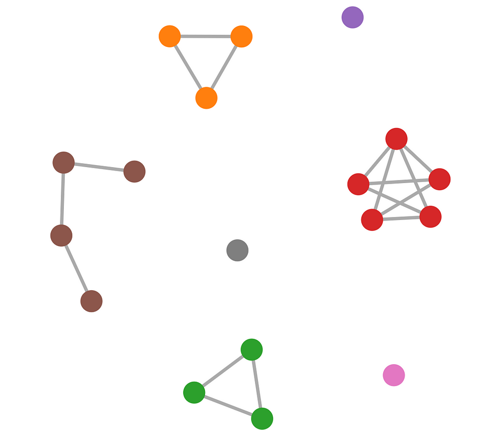
🦚 Note: In the example, you can see a disconnected graph with 7 connected components, 3 of which are isolated vertices in the sense that there is no vertex in the component that isn’t connected to it and no “outside” vertex connected to it.

In simpler terms, it’s a self-contained group of interconnected vertices. This means that, with the interactive visualization, we can see how disconnected graphs have multiple connected components. For the point cloud scenario, each connected component corresponds to a potential object. By identifying these connected components, we can effectively segment the point cloud into meaningful clusters.

🦚 Note: If you want to explore graph theory interactively, I highly recommend using the online tool “d3-graph-theory” (https://d3gt.com/). It allows for interactive graph manipulation to illustrate many very useful concepts.

Now that you have a solid foundation for understanding how we transform the unstructured point cloud data into a structured graph representation, let us enable it with Python.

The Python Function Definition

We introduce a sophisticated graph construction method build_radius_graph() that transforms point cloud data into a networked representation. The function utilizes a KDTree for efficient spatial querying, connecting points within a specified radius and optionally limiting the number of neighbors per node. 

def build_radius_graph(points, radius, max_neighbors):
    
    # Convert points to numpy array if not already
    points = np.asarray(points)
    
    # Create KD-tree
    kdtree = KDTree(points)
    
    # Initialize graph
    graph = nx.Graph()
    
    # Add nodes with position attributes
    for i in range(len(points)):
        graph.add_node(i, pos=points[i])
    
    # Query the KD-tree for all points within radius
    pairs = kdtree.query_pairs(radius)
    
    # Add edges to the graph with distances as weights
    for i, j in pairs:
        dist = np.linalg.norm(points[i] - points[j])
        graph.add_edge(i, j, weight=dist)
    
    # If max_neighbors is specified, prune the graph
    if max_neighbors is not None:
        prune_to_k_neighbors(graph, max_neighbors)
        
    return graph

By using NetworkX’s graph structure, we create a flexible framework for topological analysis that captures local spatial relationships.

The KD-Tree plays a pivotal role in establishing connections between points in the point cloud. For each point, we query the KD-Tree to find its neighbors within a defined radius. These neighbors are the candidates for edge creation in our graph. The efficiency of the KD-Tree allows us to perform these neighbor searches rapidly, even for large point clouds.

The approach shines here: we leverage the KD-Tree neighbor searches to build our graph. Each point in the point cloud becomes a node in the graph. An edge is created between two nodes if and only if they are identified as neighbors within the specified radius during the KD-Tree search. Let’s put this “parameter” on hold to explore it with the dataset at hand.

The pruning function

Finally, as you can see, I define an accompanying prune_to_k_neighbors() function that implements a critical graph refinement technique. 

This ensures that each node maintains only its k-nearest neighbors, effectively controlling graph complexity and reducing computational overhead.

def prune_to_k_neighbors(graph, k):
    for node in graph.nodes():
        edges = [(node, neighbor, graph[node][neighbor]['weight'])
                for neighbor in graph[node]]
        if len(edges) > k:
            # Sort edges by weight
            edges.sort(key=lambda x: x[2])
            # Remove edges beyond k nearest
            edges_to_remove = edges[k:]
            graph.remove_edges_from([(e[0], e[1]) for e in edges_to_remove])

simulation_graph = build_radius_graph(xyz, radius=0.1, max_neighbors=4)

This pruning mechanism is particularly valuable in high-dimensional point clouds where unconstrained graph construction could lead to exponential complexity, making our approach both computationally efficient and topologically meaningful.

Beautiful! We now have a way to generate graphs, so naturally, let’s put it to the test! For this, let me first generate some dummy data (a 2D point cloud):

np.random.seed(42)
n_points = 300
xyz = np.random.rand(n_points, 2)

We can now use the xyz point cloud for some 2D tests. It is an array as follows:

array([[0.37454012, 0.95071431],
       [0.73199394, 0.59865848],
       [0.15601864, 0.15599452],
       [0.05808361, 0.86617615],
                ...
       [0.60111501, 0.70807258],
       [0.02058449, 0.96990985],
       [0.83244264, 0.21233911],
       [0.18182497, 0.18340451]])

Let us use our defined function with a radius = 0.1 and 4 neighbors:

simulation_graph = build_radius_graph(xyz, radius=0.1, max_neighbors=4)

Now, if you try to call your simulated graph, you would get that:

<networkx.classes.graph.Graph at 0x1e86ec99460>

This means our function works! And from the Graph class, you can explore the nodes (simulation_graph.edges()), or the edges (simulation_graph.edges()) for example:

#For the nodes, you would get:
NodeView((0, 1, 2, ...))

#For the edges, you would get:
EdgeView([(0, 205), (0, 197), ...])

but no way to extract its key characteristics? Let us solve this by proposing an analytical step.

Step 3. Graph Analytics for Euclidean Clustering

We want to use the concepts highlighted in the graph theory (connected components) for our analytical tasks. To this end, we construct a analyze_components() function that provides a comprehensive statistical graph connectivity analysis. 

def analyze_components(graph):

    components = list(nx.connected_components(graph))
    
    analysis = {
        'num_components': len(components),
        'component_sizes': [len(c) for c in components],
        'largest_component_size': max(len(c) for c in components),
        'smallest_component_size': min(len(c) for c in components),
        'avg_component_size': np.mean([len(c) for c in components]),
        'isolated_points': sum(1 for c in components if len(c) == 1)
    }
    
    return analysis

By computing metrics such as the number of components, their sizes, and the count of isolated points, we gain deep insights into the topological structure of our point cloud. These metrics are essential for understanding the dataset’s spatial distribution and clustering characteristics. Let put it to the test.

component_analysis = analyze_components(simulation_graph)
print("\nComponent Analysis:")
for metric, value in component_analysis.items():
    print(f"{metric}: {value}")

This returns:

Component Analysis:
num_components: 9
component_sizes: [169, 10, 32, 43, 2, 23, 11, 5, 5]
largest_component_size: 169
smallest_component_size: 2
avg_component_size: 33.333333333333336
isolated_points: 0

As you can see, the analysis reveals critical information about graph topology: how many distinct clusters exist, their relative sizes, and the presence of isolated points. This approach transforms raw geometric data into a rich, quantitative description of spatial relationships, which we can now leverage for further processing of our point cloud.

Now, let us plot our graphs.

Step 4. Plotting Euclidean Clustering Graphs (Optional)

You can define a plot_components() function for a sophisticated graph-based point cloud representation visualization technique. At this stage, you should be deep enough into Python code that creating such a function is a great exercise to master Python for 3D. To help you on that front, I encourage you to first get the connected components, create a color iterator, create a figure that you populate iterating on the components.

Here is some sample code to help you get started:

    # Get connected components
    components = list(nx.connected_components(graph))
    n_components = len(components)
    
    # Create color iterator
    colors = plt.colormaps[cmap](np.linspace(0, 1, max(n_components, 1)))

By color-coding connected components and rendering their edges and nodes, we can then create an intuitive visual representation of graph topology. 

🦚 Note: The best is to design a visualization strategy using matplotlib’s color mapping to distinguish between different graph components, providing an immediate visual understanding of spatial clusters. By dynamically generating colors based on the number of components and rendering edges with varying transparencies, we can create a pleasing representation of graph structure.

Step 5. Connected Components for Point Clouds

Let us use our synthetic point cloud data to demonstrate graph construction and analysis techniques (I used random point generation with a fixed seed for reproducibility). The algorithm we use to identify clusters is connected component analysis. This fundamental graph algorithm efficiently finds all connected components within a graph. 

As a reminder, a connected component is a maximal subgraph where every pair of nodes is connected by a path. In our context, each connected component represents a potential object in the scene. NetworkX, our chosen Python library for graph manipulation, provides efficient implementations of connected component analysis that we leverage.

We create controlled scenarios to explore graph behavior under different parameters). The code systematically varies radius and neighbor count, allowing us to observe how these parameters influence graph topology.

🦚 Note: The simulation approach is a powerful method for understanding graph construction algorithms. By exploring parameter sensitivity through controlled experiments, we can develop robust graph-based clustering strategies that are adaptable to diverse point cloud characteristics. 

Parameter’s Analysis

The Radius parameter

The radius acts as a crucial parameter, controlling the granularity of the clustering. Let us check and vary the parameter by executing this Python code snippet:

for radius_simulation in [0.05,0.1,0.5]:
    simulation_graph = build_radius_graph(xyz, radius=radius_simulation, max_neighbors=5)
    plot_components(simulation_graph, xyz, radius_simulation, 5)
    plt.show()

A smaller radius will result in more fragmented clusters, while a larger radius will produce fewer, more interconnected clusters (see below). 

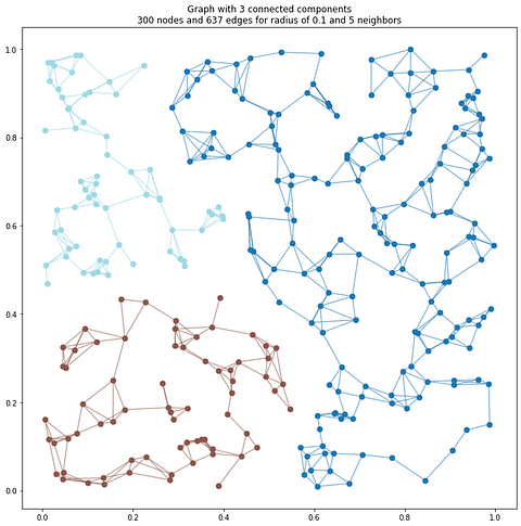
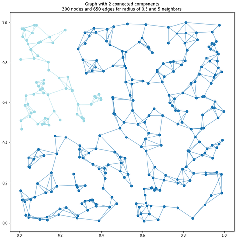
As you can see, by defining a fixed spatial distance, we control the local neighborhood interactions, essentially creating a topological constraint that captures the intrinsic geometric relationships within the dataset. This parameter’s sensitivity directly impacts cluster formation, with smaller radii potentially fragmenting the point cloud into numerous small components and larger radii risking over-merging distinct spatial structures.

🌱 Growing: A small radius results in highly localized connectivity, which leads to the formation of numerous small, fragmented clusters. This approach can be beneficial for isolating fine details; however, it also raises the likelihood of over-segmentation, which may result in dividing a single object into several clusters due to noise or differences in sampling density. A larger radius leads to wider connections, which may lead to the merging of separate objects, particularly in cluttered environments where objects are closely situated. The optimal radius is significantly influenced by the data available.

The maximum neighbors parameter

We also introduce a pruning step, limiting the maximum number of edges connected to each node. This prevents over-connectivity in dense regions, ensuring that the resulting clusters reflect meaningful object boundaries. To check the parameter’s influence, let us use this Python code:

for neighbors_simulation in [2,5,10]:
    simulation_graph = build_radius_graph(xyz, radius=0.1, max_neighbors=neighbors_simulation)
    plot_components(simulation_graph, xyz, 0.1, neighbors_simulation)
    plt.show()

Let us explore how the max_neighbors parameter influences our results:

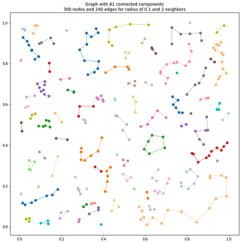
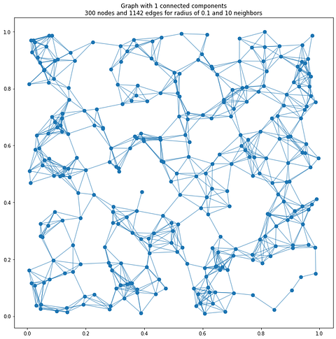
The max_neighbors parameter acts as a computational and topological regularization mechanism, preventing excessive graph complexity by limiting the number of connections per node. 

As we see, this parameter introduces a critical trade-off between local representational fidelity and global graph interpretability. 

Too few neighbors might disconnect meaningful spatial relationships, while too many could introduce noise and reduce the discriminative power of the graph representation. Selecting optimal values requires iterative experimentation, considering the specific geometric characteristics of the point cloud and the intended analytical objectives.

This methodology is critical in developing generalizable algorithms for spatial data analysis. Now that we have everything that seems to work on our simulated dataset let us cluster our 3D Point Cloud.

Step 6. Euclidean Clustering for 3D Point Clouds

We want to leverage our graph structure for Euclidean clustering. The idea is that we use the distance between points defined as the Euclidean distance (straight-line distance) between their 3D coordinates. This is a natural choice for many applications, as it reflects the spatial proximity of points in the real world. However, other distance metrics, such as Manhattan distance or geodesic distance, can be used depending on the application’s specific requirements. You can check the 3D Segmentor OS Course to extend your knowledge.

Transitioning from simulated to real-world data, we construct a graph using the actual point cloud dataset. The innovative approach here is computing the graph’s radius based on the point cloud’s nearest neighbor distance, creating a data-driven connection strategy. 

# Visualizing our input point cloud
o3d.visualization.draw_geometries([pcd])

# Get point cloud coordinates
xyz = np.asarray(pcd.points)
nn_d = np.mean(pcd.compute_nearest_neighbor_distance()[0])

We adaptively capture local spatial relationships by scaling the radius to three times the average nearest neighbor distance. Then, we can use our graph construction process to demonstrate our approach to point cloud analysis. 

# Build the graph
graph = build_radius_graph(xyz, radius=nn_d*3, max_neighbors=10)

# Analyze components
component_analysis = analyze_components(graph)
print("\nComponent Analysis:")
for metric, value in component_analysis.items():
    print(f"{metric}: {value}")

Graph Analysis

We can extract meaningful structural information by analyzing the connected components in the real-world dataset, potentially identifying distinct object segments or spatial clusters within the point cloud.

Component Analysis:
num_components: 52
component_sizes: [5836, 743, 214, 6, 1, 2, 1, 1, 1, 16771, 1935, 3567, 1872, 16, 266, 1359, 352, 1648, 8792, 1246, 2710, 81, 74, 47, 5, 18, 8, 13, 1, 3, 14, 4, 8, 1, 2, 8, 2, 1, 7, 2, 8, 1, 1, 1, 2, 2, 1, 1, 1, 1, 1, 1]
largest_component_size: 16771
smallest_component_size: 1
avg_component_size: 916.5192307692307
isolated_points: 16

 We can see that we have 52 main components, 16 of which are isolated points. The average size is 917 points, with the biggest (likely the bed) being 16 771 points.

Finally, let us visualize the results of our clustering. For this, let us create plot_cc_o3d(), a specialized function for visualizing connected components in 3D point clouds using Open3D. 

def plot_cc_o3d(graph, points, cmap = 'tab20'):
    
    # Get connected components
    components = list(nx.connected_components(graph))
    n_components = len(components)
    
    # Create color iterator
    colors = plt.colormaps[cmap](np.linspace(0, 1, max(n_components, 1)))
    rgb_cluster = np.zeros(np.shape(points))
    
    # Plot each component with a different color
    for idx, component in enumerate(components):
        if len(component)<=10:
            rgb_cluster[list(component)] = [0, 0, 0]
            idx-=1
        else:               
            color = colors[idx][:3]
            rgb_cluster[list(component)] = color
    
    pcd_clusters = o3d.geometry.PointCloud()
    pcd_clusters.points = o3d.utility.Vector3dVector(xyz)
    pcd_clusters.colors = o3d.utility.Vector3dVector(rgb_cluster)
    return pcd_clusters

By color-coding components and handling small clusters differently, we create a nuanced visualization that highlights significant spatial structures while minimizing visual clutter from minor components.

The implementation is particularly clever in its handling of small clusters, assigning them a neutral color to distinguish them from major components. This approach provides a clear, informative visualization that helps researchers quickly understand the spatial organization of complex point cloud datasets, bridging computational analysis with intuitive visual interpretation. Now let us leverage and plot our scene:

pcd_cluster = plot_cc_o3d(graph, xyz)
pcd_cluster.estimate_normals()
o3d.visualization.draw_geometries([pcd_cluster])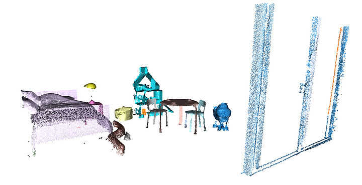

The results of the Euclidean clustering demonstrated on the real-world point cloud are particularly compelling due to their effectiveness in a practical scenario. We can see that the algorithm successfully isolates individual furniture pieces, including the bed, chairs, table, lamps, basket, and even small toys within the dollhouse. 

This ability to delineate object boundaries, even in a cluttered scene with varying object sizes and shapes, showcases the approach’s robustness. Notably, it handles overlapping objects like the chair and table, separating them into distinct clusters despite the overlap in the top-down view.

This is wonderful! Now, let us analyze a bit how we could extend the solution.

Euclidean Clustering: Discussion and perspectives

One of the most significant advantages of this approach is its automation. The entire process, from graph construction to cluster visualization, is automated within a Python script. This eliminates the need for manual segmentation, significantly saving time and effort. 

Additionally, the clustering process inherently acts as a noise reduction technique. Small, isolated clusters, often representing noise or spurious points, are filtered out, leaving behind more substantial clusters representing actual objects.

The scalability and efficiency of the KD-Tree for neighbor searches with the connected component analysis algorithm allow for the processing of large, complex point clouds. This opens up possibilities for applications in urban mapping, 3D modeling, and robotics.

Perspectives

The segmented clusters serve as a solid foundation for further analysis. By extracting features like size, shape, position, and orientation from each cluster, we can enable object recognition, scene understanding, and other downstream applications. For example, in a point cloud representing a colored object, integrating color information into the edge weights can assist in distinguishing between spatially close areas yet exhibit different colors. Additionally, advanced graph algorithms like spectral clustering and community detection can reveal higher-level relationships among clusters, facilitating scene understanding and object recognition.

The next logical step is implementing a classifier on top of these segmented clusters to automate object identification and categorization.

🌱 Growing: This flexible and efficient framework allows us to move beyond Euclidean clustering. By incorporating attributes beyond just spatial proximity (e.g., color, intensity, or normal vectors) into the edge weighting scheme, we can significantly improve the robustness and accuracy of the segmentation. Furthermore, advanced graph algorithms like community detection can be applied to identify higher-level relationships between clusters, uncovering hierarchical structures within the point cloud data. This opens up exciting possibilities for scene understanding and object recognition in diverse 3D applications.

Conclusion

In conclusion, the results demonstrate the practical utility of graph-based Euclidean clustering for real-world point cloud segmentation. Its automated nature, robustness to complex scenes, noise reduction capabilities, and scalability make it a powerful tool for extracting meaningful information from 3D data. We transform point clouds into meaningful object representations by leveraging KD-Trees for neighbor searches and connected component analysis for cluster identification.

The effectiveness of graph-based Euclidean clustering is found in its capacity to convert the unstructured characteristics of point cloud data into a structured and analyzable format. Nevertheless, this capability entails the obligation of precise parameter adjustment and a detailed comprehension of the procedure. 

The result of our clustering procedure is a collection of segmented point cloud clusters. Nonetheless, the primary objective is frequently to recognize and classify these clusters as distinct entities. This necessitates the incorporation of classification methods, which may be either supervised or unsupervised.

🌱 Growing: From a computational geometry perspective, graph representations transform point clouds into powerful topological networks that capture intrinsic spatial relationships. By encoding geometric information as a graph, we enable advanced analyses such as feature extraction, connectivity analysis, and semantic segmentation. For instance, in urban mapping, these graphs can represent not just spatial proximity but semantic relationships between building structures, infrastructure, and terrain. The graph’s edge weights and connectivity patterns become informative features for machine learning models, allowing us to train algorithms that understand spatial context beyond mere point coordinates.

About the author

Florent Poux is a Scientific and Course Director focused on educating engineers on leveraging AI and 3D Data Science. He leads research teams and teaches 3D Computer Vision at various universities. His current aim is to ensure humans are correctly equipped with the knowledge and skills to tackle 3D challenges for impactful innovations.

Resources

1. 🏆Awards: Jack Dangermond Award
2. 📕Book: 3D Data Science with Python 
3. 📜Research: 3D Smart Point Cloud (Thesis)
4. 🎓Courses: 3D Geodata Academy Catalog
5. 💻Code: Florent’s Github Repository
6. 💌3D Tech Digest: Weekly Newsletter

🦊 Florent: If you want to deepen your skills, I recommend the comprehensive course “Segmentor OS. ” In it, we implement these concepts hands-on and explore advanced optimization techniques for real-world projects.

Other 3D Tutorials

You can pick another Open-Access Tutorial to perfect your 3D Craft.

• Python Guide for Euclidean Clustering of 3D Point Clouds
• A Quick Dive into Modern Point Cloud Workflow
• 3D Mesh from Point Cloud: Python with Marching Cubes Tutorial
• How to Quickly Visualize Massive Point Clouds with a No-Code Framework
• Building a 3D Object Recognition Algorithm: A Step-by-Step Guide
• 3D Generative AI: 11 Tools (Cloud) for 3D Model Generation
• 3D Shape Detection with RANSAC and Python (Sphere and Plane)
• Tutorial for 3D Semantic Segmentation with Superpoint Transformer
• 3D Python Environment Setup: 7-Steps Guide for Beginners
• 2D Image to 3D Model
• 3D Point Cloud to Voxels: Python Voxelization Tutorial
• 3D Gaussian Splatting: Hands-on Course for Beginners
• 3D Reconstruction from a Single Image: Tutorial
• 3D Deep Learning Essentials: Ressources, Roadmaps and Systems
• Point Cloud Feature Extraction: Complete Guide