
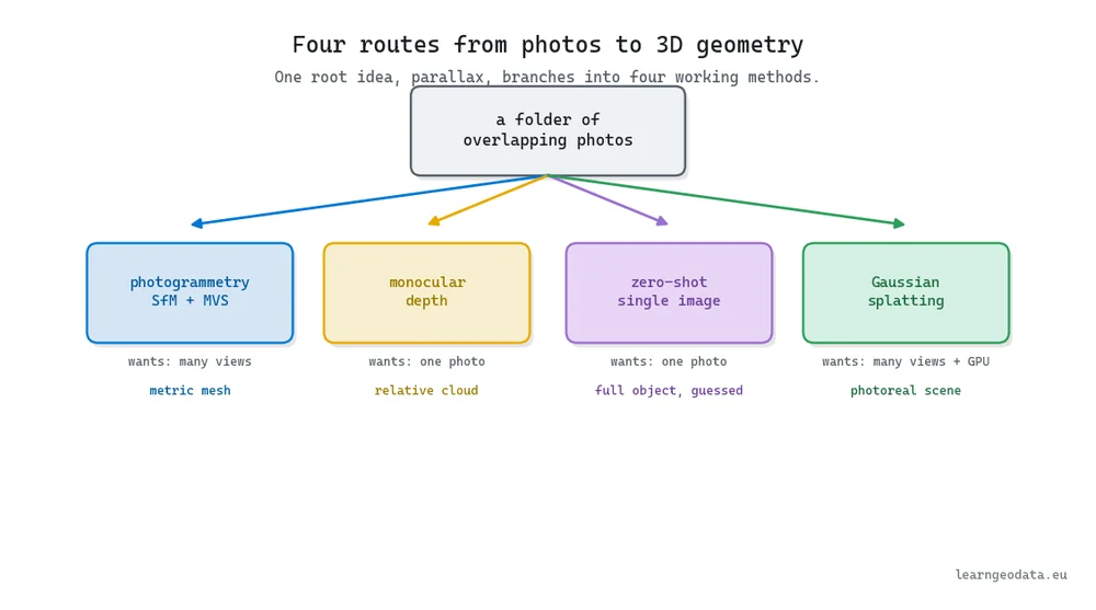
3D reconstruction turns ordinary photographs into geometry you can measure and hand off, with no laser scanner involved. Four routes reach it: classical photogrammetry through COLMAP or Meshroom, monocular depth back-projected in Open3D, single-image models, and Gaussian splatting. Parallax is the one idea under all four, and overlap decides whether any of them work.
Open your camera roll and there’s a fair chance a 3D model is already sitting in it. Forty shots of a statue. A walk around your kitchen.
| What it is | Rebuilding measurable 3D geometry from ordinary photos, by four routes: photogrammetry, monocular depth, single-image models, and Gaussian splatting |
| What you build | A textured mesh from a folder of photos driven by COLMAP, plus a point cloud back-projected from one photo’s depth map in Open3D |
| Libraries | COLMAP and AliceVision or Meshroom, Open3D, NumPy, Depth Anything v2 for monocular depth |
| Who it is for | Anyone with a camera and Python who wants usable 3D without buying a scanner |
| Level | Beginner to intermediate. The working numbers are 30 to 50 frames for a small object and 60 to 80 percent overlap. |
Here is the path this guide takes, so you can jump straight to the part you need:
- What 3D Reconstruction Actually Is And Why It Matters
- Parallax The One Idea Under Every 3D Reconstruction
- The Classical 3D Reconstruction Pipeline Stage By Stage
- How Many Photos And How Much Overlap
- Turning A Single Photo Into Depth With Open3D
- Why Gaussian Splatting Reset The Realism Bar
- How To Choose A 3D Reconstruction Method Before You Shoot
- Recovering Real Scale And The Pitfalls That Bite
- Where This Fits And Where To Go Next
- Build Your First Reconstruction This Week
- Frequently Asked Questions
Each of those folders holds enough information to rebuild the scene in three dimensions, and you don’t need a scanner or a lab to pull it out. This is the complete guide to 3D reconstruction, the practice of turning flat pictures into geometry you can measure, rotate, and hand to someone else.
Here’s a thing that always makes me smile. In 1838, the astronomer Friedrich Bessel measured how much a faint star called 61 Cygni shifted against the background as Earth moved around the Sun. From that tiny shift, he calculated the distance to a star for the first time in history. He never left the ground, yet he measured light-years.
That measurement and the reconstruction you’re about to build run on the exact same trick. Move your viewpoint, watch how things shift, and the shift tells you distance. So if an astronomer could measure a star from two positions, what can a laptop do with a folder of photos?
What you’ll learn in this article:
- The single idea (parallax) that makes photos reconstructable, and why overlap decides everything
- How structure from motion and multi-view stereo rebuild a mesh, stage by stage
- Where AI monocular depth fits, with real Open3D code that back-projects one photo into points
- What Gaussian splatting changed about realism, and when a plain mesh still wins
- A blunt rule for picking a 3D reconstruction method before you shoot a single frame
Estimated reading time: 13 minutes
What 3D Reconstruction Actually Is And Why It Matters
Strip away the jargon and 3D reconstruction is one sentence: it turns ordinary images into 3D geometry, without you buying a laser scanner. That geometry might be a point cloud, a triangle mesh, or a cloud of translucent blobs, but the shape is what matters.
Why should you care? Because that one skill sits underneath a surprising amount of work. A heritage team documents a crumbling facade from a phone. A game studio fills a level with props scanned off real objects. A robotics group builds training scenes from an ordinary camera.
All of them face the same first problem, which is getting reality into the machine. Reconstruction is one of the two doors into that machine, and firing a laser is the other.
So the payoff here is not academic. Get reconstruction right and everything downstream inherits a clean foundation.
Parallax The One Idea Under Every 3D Reconstruction
Parallax is the one idea under every 3D reconstruction, and the rest of this page is variations on it. When you move a camera, near things slide further across the frame than far things do. Your brain reads that differential shift as depth every time you walk down a hallway, and a reconstruction algorithm reads it the same way.
Hand it two photos of a wall taken from slightly different spots, and the distance each point slid tells you how far away that point sat. That’s Bessel’s stellar shift, brought down to desk scale.
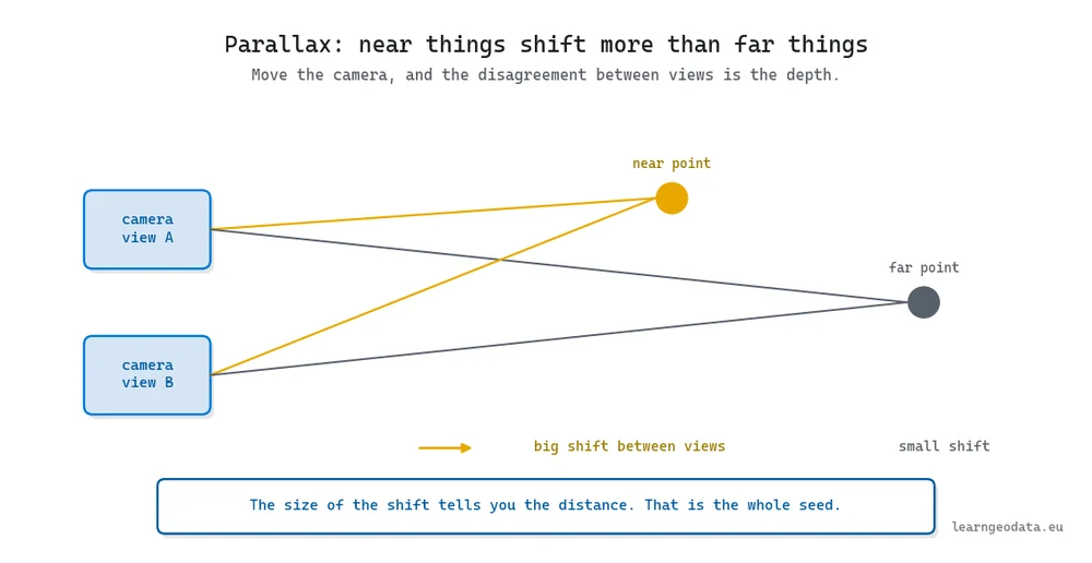
So the raw material of reconstruction isn’t really the pixels. It’s the disagreement between views. That’s why one flat photo is hard and a folder is easy: more viewpoints mean more disagreement to triangulate from.
It also explains the first rule you’ll break exactly once and then never again. Your photos have to overlap, and they have to overlap generously.
🦥 Geeky Note: A classical pipeline matches keypoints between images before it attempts anything three-dimensional. COLMAP pulls up to 8192 SIFT keypoints per photo by default, and it can only place a camera when enough of those keypoints reappear in the neighbouring shots. Practical target: keep roughly 70 percent of each frame visible in the next one, and shoot 30 to 50 images for a tabletop object. Starve the matcher of shared points and cameras either drift or refuse to register.
The Classical 3D Reconstruction Pipeline Stage By Stage
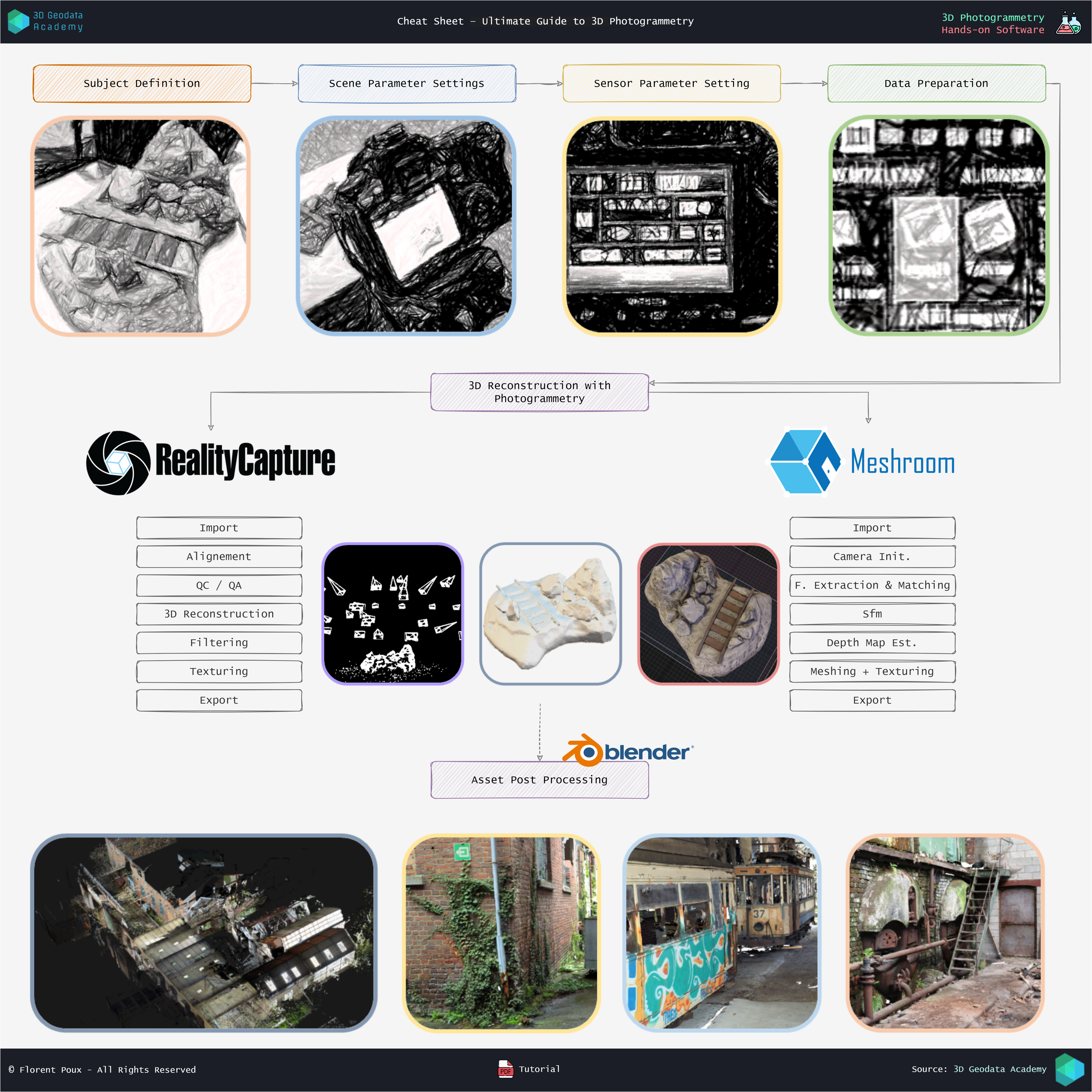
Start with the classical route, because it hands you the words every later method reuses. You feed an algorithm a stack of overlapping photos and it works in two acts.
The first act, structure from motion, figures out where each camera stood and produces a thin, sparse cloud of the points it was confident about. The second act, multi-view stereo, revisits those solved cameras and fills the gaps until the cloud is dense enough to wrap a surface around.
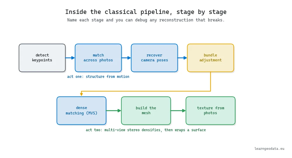
That two-act structure hasn’t gone anywhere, and it’s worth being able to name each stage. If a reconstruction comes back warped or doubled, you’ll know whether the poses were wrong (an act-one problem) or the densification smeared (an act-two problem).
Tools like COLMAP and the open AliceVision stack run this exact chain, and the neural methods later on quietly call the same pose step under the covers. So this vocabulary is not throwaway theory. It’s the map you’ll navigate by. For the full photo-to-model workflow laid out stage by stage, see our 3D reconstruction pipeline guide.
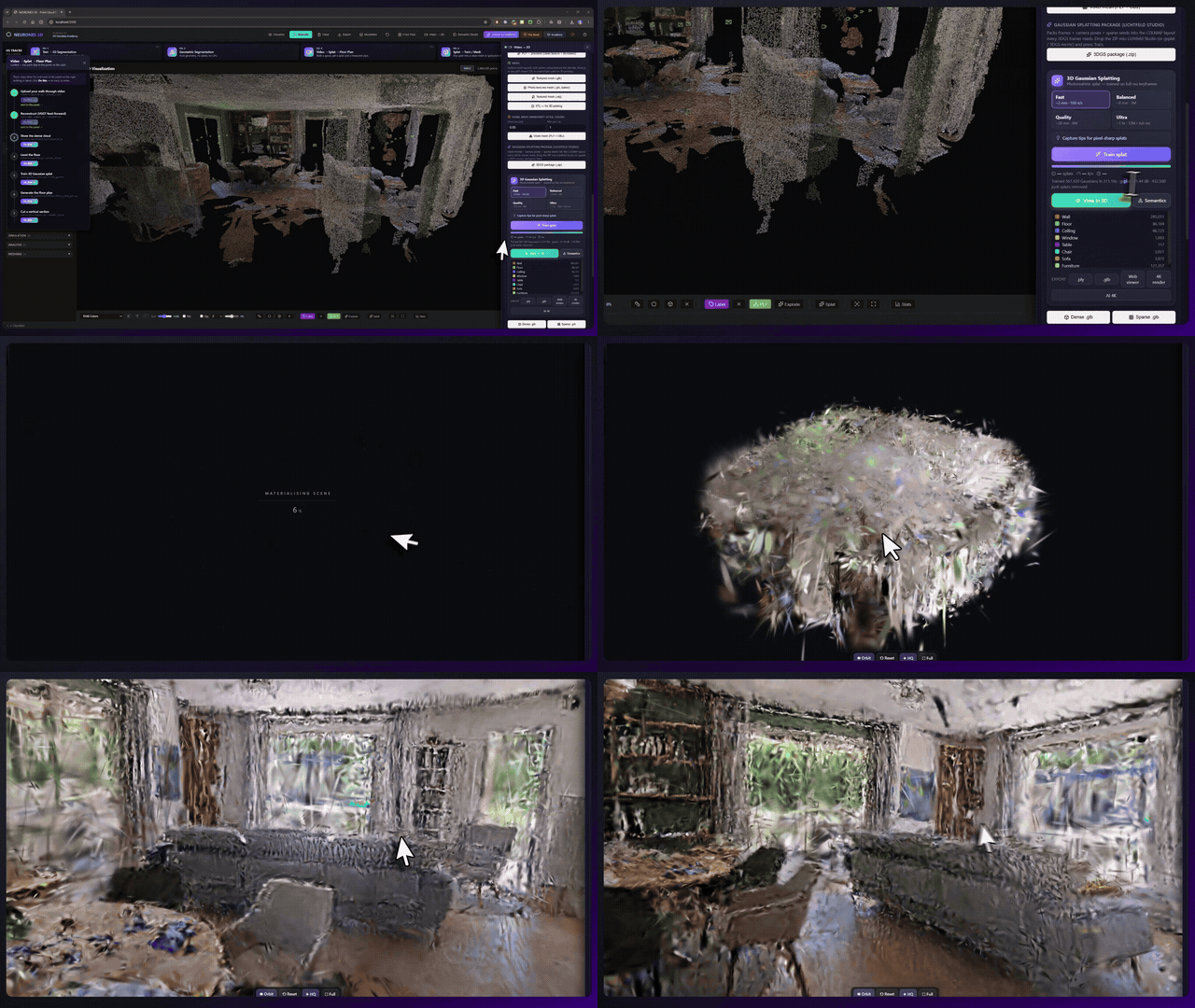
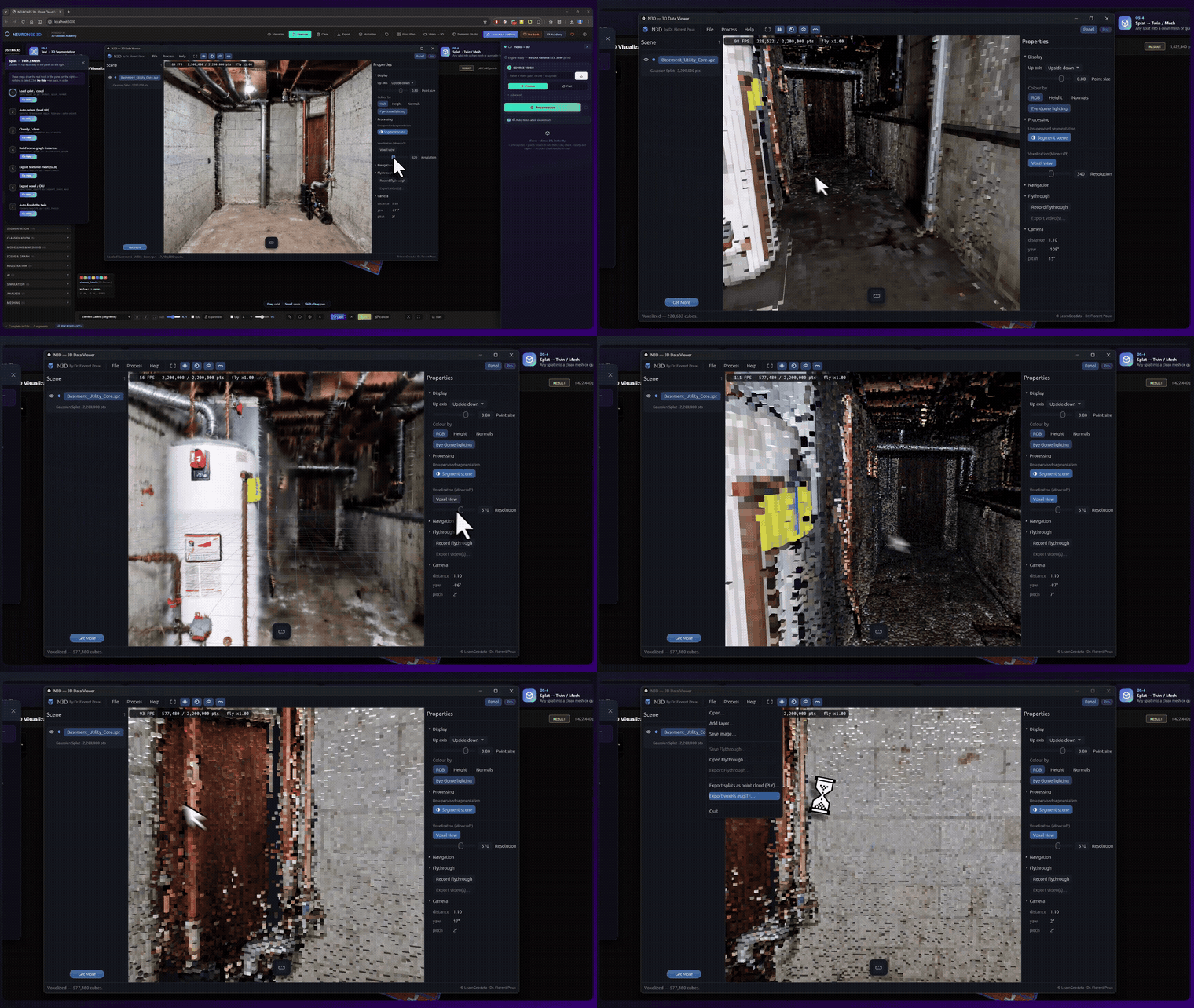
If you want the fastest way onto the board, drive Meshroom, the graphical front end for AliceVision. Point it at a folder, press start, and pull a textured mesh out the other side without hand-tuning a hundred sliders. Once you outgrow clicking, the same pipeline scripts headlessly, which is where the real automation lives.
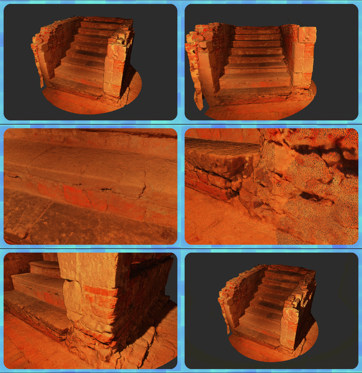
That headless route is worth seeing, because it turns the whole two-act chain into a single call you can drop in a loop. COLMAP ships an automatic_reconstructor that runs every stage you just named, from feature detection through dense meshing, behind one command. Driving it from Python with subprocess keeps the entire job, photos in and mesh out, inside a script you control.
import subprocess
from pathlib import Path

# One folder of overlapping photos in, a solved project (sparse + dense) out.
project = Path("reconstruction/statue")
images = project / "images"
project.mkdir(parents=True, exist_ok=True)

# automatic_reconstructor chains the full classical pipeline in one call:
# feature extraction, matching, SfM poses, MVS densification, then meshing.
subprocess.run(
    [
        "colmap", "automatic_reconstructor",
        "--workspace_path", str(project),
        "--image_path", str(images),
        "--data_type", "individual",   # unordered photos, not a video sequence
        "--quality", "high",           # spend more minutes for a denser result
        "--dense", "1",                # run multi-view stereo, not just SfM
    ],
    check=True,   # raise if COLMAP exits non-zero, so a failure never passes silently
)

# The dense cloud and Poisson mesh land under the workspace, ready for Open3D.
print("done ->", project / "dense" / "0" / "meshed-poisson.ply")
That single call hides a lot of moving parts, and that is the point. When it works you get a mesh; when it fails, you now know which named stage to interrogate. The --quality flag is the honest lever, since higher settings simply trade more minutes for more points.
🦚 Florent’s Note: Classical photogrammetry is picky about three things, and it will punish you for ignoring any of them: texture, sharpness, and overlap. Point it at a mirrored office facade and watch the reconstruction dissolve into holes, because a glass panel looks completely different from every angle and structure from motion assumes a point looks the same from all of them. A wall of matte brick, by contrast, reconstructs almost too easily. When a scan fails, the software is rarely the culprit. The surface is.
How Many Photos And How Much Overlap
Let me answer the question everyone actually asks first: how many photos? For a single object on a table, 30 to 50 sharp frames walked in a slow circle is a safe start. For a room or a building, you’ll want more, and you’ll want to think about coverage rather than raw count.
But the count matters less than the overlap, and this is where beginners lose whole afternoons. Two neighbouring photos need to share a big chunk of the scene, so the matcher finds the same physical points in both.
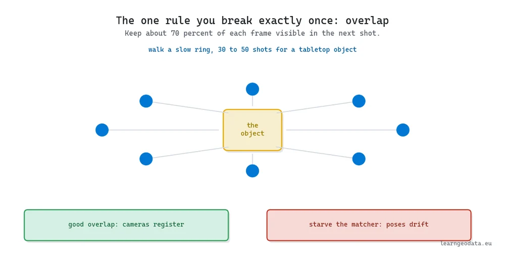
Think of it like laying bricks. Each new photo has to bond to the one before it, and if you leave a gap, the wall cracks right there.
So resist the urge to take four dramatic photos from the corners of the room. Take twenty boring ones with heavy overlap instead. Boring wins.
🦥 Geeky Note: Bundle adjustment is the quiet workhorse that makes or breaks the geometry. It tunes all the camera poses and all the 3D points together to shrink the reprojection error, the gap in pixels between where a point actually lands and where the current guess puts it. Keep 60 to 80 percent overlap between neighbours, which hands the solver plenty of common observations to pin things down. Drop below that and the error surface turns flat and ambiguous, and your cloud comes back bent.
Turning A Single Photo Into Depth With Open3D
Everything so far demanded many views and honest parallax. But be honest about your own photo library: much of it is one-off shots with no sibling frame anywhere. A single photo of a building. One product image off a listing.
So the field asked the obvious thing: what if one image were enough? A monocular depth model answers that by predicting a depth value for every pixel, trained on a huge pile of scenes until it has absorbed how the world tends to be laid out. Send those per-pixel depths back out along the camera rays and one photo becomes a full point cloud. Our single-image 3D reconstruction tutorial walks this route on its own.
Depth Anything v2 is one of the stronger open models for this, and it picks up exactly where the many-view methods run dry. But how does a flat depth map actually become 3D points? That step is called back-projection, and doing it by hand once is the best way to understand what a depth map really is.
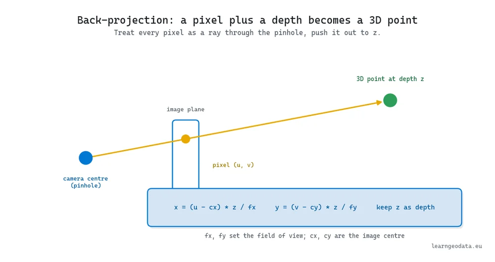
The geometry is short. Once a model hands you the array of predicted depths, you unproject each pixel: treat it as a ray through the pinhole camera, then push that ray out to its predicted distance. Open3D gives you a clean container for this, and it can do the whole unprojection in one call once you supply the camera intrinsics.
import numpy as np
import open3d as o3d

# depth: an H x W array of predicted distances from a monocular model
depth = np.load("depth_prediction.npy").astype(np.float32)
h, w = depth.shape

# Wrap the raw depth array as an Open3D image.
depth_o3d = o3d.geometry.Image(depth)

# Pinhole intrinsics. With no EXIF focal length, start near the image width.
fx = fy = 1.2 * w
cx, cy = w / 2.0, h / 2.0
intrinsic = o3d.camera.PinholeCameraIntrinsic(w, h, fx, fy, cx, cy)

# Open3D shoots one ray per pixel and lands it at the predicted depth.
cloud = o3d.geometry.PointCloud.create_from_depth_image(
    depth_o3d,
    intrinsic,
    depth_scale=1.0,      # model output already reads as depth units
    depth_trunc=1000.0,   # ignore anything beyond this distance
    stride=1,
)

o3d.io.write_point_cloud("single_photo_cloud.ply", cloud)
The one number that governs this whole block is the focal length, fx. A real photo carries it in EXIF metadata. A random image off the internet does not, so the 1.2 * w guess sets the field of view for you.
Get it wrong and the cloud stretches or squashes along the depth axis. Feed a metric focal and a metric depth and the points land in real metres. Guess both, and the shape comes out right while the size stays relative.
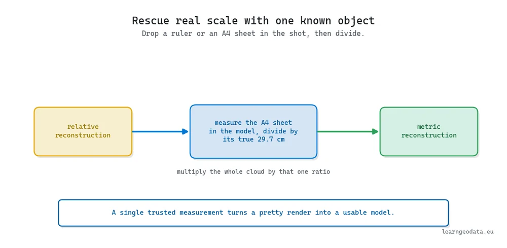
🌱 Growing Note: You can claw back real scale without a full survey. Drop one object of known size into the shot, a 30 centimetre ruler or a standard A4 sheet at 29.7 centimetres tall, then divide the reconstructed length of that object by its true length and multiply the whole cloud by the ratio. A single trusted measurement converts a relative reconstruction into a metric one, which is often the difference between a pretty render and a usable model.
🪐 System Thinking Note: Watch the same trade repeat as you move down this page. Classical multi-view stereo hands you metric accuracy but asks for many calibrated views. Learned methods loosen the input, sometimes down to one frame, and give back geometry that looks right rather than geometry that was measured. Neither is the winner. A survey needs the millimetres; a game background needs the look. Judge by what your task can live with.
Why Gaussian Splatting Reset The Realism Bar
Gaussian splatting reset the realism bar by holding photographic realism without locking you into either a tidy mesh or a flat depth map. The classical route buys accuracy, the AI depth route buys convenience, and splatting buys the look of the photographs themselves.
The trick is to never build a surface at all. 3D Gaussian splatting (Kerbl and colleagues, 2023) builds a scene from a swarm of tiny see-through blobs, each holding a spot, a colour, and an orientation, then keeps nudging the swarm until its render lines up with your photos.
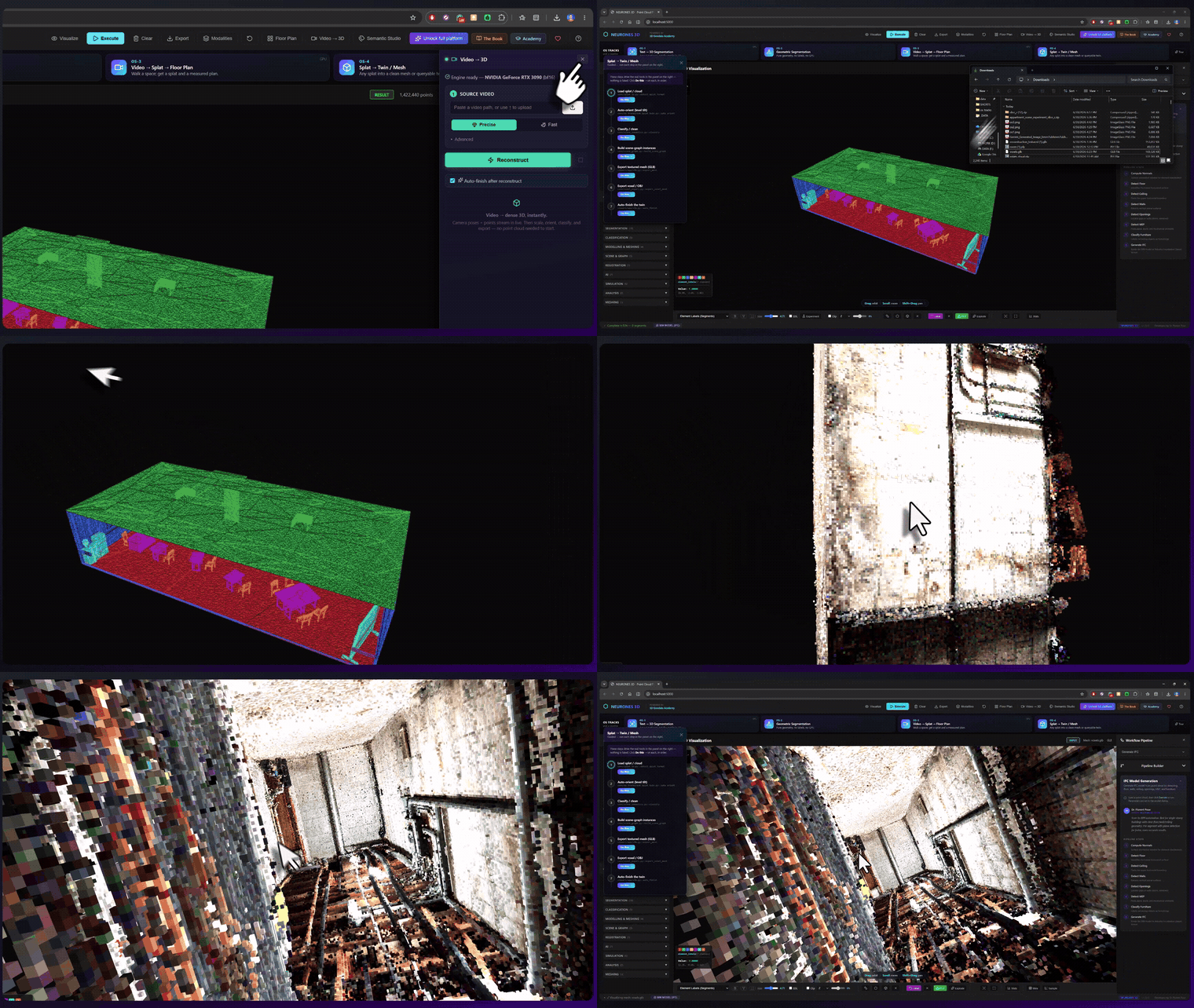
The payoff is photorealistic new viewpoints at interactive frame rates, holding reflections and fine detail a triangle mesh struggles to capture. One caveat, though. A splatting run needs camera poses first, usually from COLMAP, so the classical stages you met earlier still do the quiet groundwork before a single blob shows up.
I said the trade was accuracy versus convenience earlier, and that’s true, but splatting bends the framing. Actually, let me put that more carefully: it steps off the accuracy axis entirely. It buys realism instead, at the cost of editability.
A splat scene is gorgeous to fly a camera through and awkward to clean up, because there’s no surface to snap tools onto. So you reach for it when the look is the deliverable, not the measurement. If you want to build one yourself, our hands-on Gaussian splatting course for beginners starts from scratch.
🦥 Geeky Note: Splatting is fast because it rasterises rather than marching rays. Every blob gets flattened onto the screen and blended by opacity, so a scene of 2 to 3 million of them holds comfortably above 100 fps on one consumer GPU, where a radiance-field model of matching quality used to crawl. The cost lands elsewhere: a finished scene can weigh several hundred megabytes on disk, and trimming it down without visible damage is a craft of its own.
How To Choose A 3D Reconstruction Method Before You Shoot
Here’s the part that saves you a wasted afternoon: pick the method before you press the shutter, because each one wants a different capture. Choose after the fact and you’ll find you shot the wrong thing.
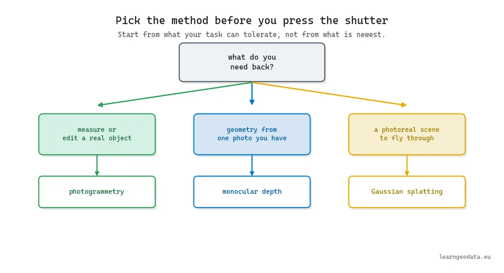
The three routes split cleanly by intent. If you need to measure or edit a real object, reach for photogrammetry and shoot 30 to 50 overlapping, sharp frames. If all you have is one image you can never re-take, run monocular depth and accept relative scale. If you want a photoreal scene to fly a camera through, capture many views and hand them to splatting.
Read that as a question about tolerance, not about which method is newest. A heritage team documenting a facade wants the measurable mesh. A previz artist filling a shot wants the splat.
And where does all of this leave the accuracy question? On a single axis, if you like it laid out plainly.
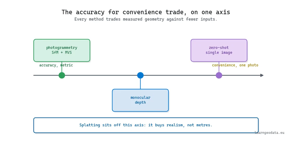
That picture is the whole strategy in one glance. You slide left for millimetres and right for convenience.
🦚 Florent’s Note: Hold onto this while you learn any of it. Plenty of apps now hand you a single button: upload photos, click, receive a 3D thing. That’s fine right up until it fails, and it always fails on the awkward job: a glare, a gap in your coverage, a surface with nothing to grip. Knowing how the machine works underneath is what lets you repair the button instead of shrugging at it. The handful of people who genuinely grasp the pipeline are the ones who get to decide what those buttons do next.
Recovering Real Scale And The Pitfalls That Bite
Let me name the traps before they cost you a project. The first is scale: a single-image reconstruction is right in shape and wrong in size, because one photo can’t tell a real chair from a doll’s chair. The fix is cheap, so put something of known size in the frame.
The second trap is reflective and textureless surfaces, and I flagged it earlier because it’s the single biggest reason hobby scans fail. Glass, chrome, a blank white wall: the matcher has nothing stable to lock onto. A light dusting of matting spray or soft diffuse lighting rescues a surprising number of these.
The third is motion blur. A sharp photo carries crisp keypoints; a blurry one smears them, and the matcher throws them out. Shoot in good light and keep the shutter fast.
The fourth is scale creep in large scenes. Over a long walk, tiny pose errors accumulate, so a corridor comes back gently banana-shaped. The cure is loop closure, revisiting a spot you already shot so the optimiser ties the ends together.
Where This Fits And Where To Go Next
Reconstruction is one of two ways reality gets into the machine. It’s the camera-based route; firing a laser is the other. Both answer the same question with different hardware, and both feed the same downstream work of making sense of the 3D data once you have it.
If you want the wider view, the 3D Spatial AI with Python guide lays out how capture, understanding, and delivery connect into one system. Two neighbours pair naturally with what you just read.
Sideways, LiDAR point cloud processing in Python is the sensor route to the same 3D points you derived here from photos. Downstream, once you hold a cloud, 3D point cloud segmentation and clustering in Python is how you split it into parts that mean something.
When you’re ready to learn the whole craft properly, with production code and the hands-on parameter feel that a single web page can’t hand you, that lives in the 3D AI Program. It’s where reconstruction stops being a party trick and becomes a system you own.
Build Your First Reconstruction This Week
Reading about parallax is not what makes it click. Building one thing is.
So pick a single object on your desk, walk a slow circle around it, and take thirty sharp, overlapping photos. Run them through Meshroom and pull out your first textured mesh before the day is over. That one small reconstruction shows you how overlap, sharpness, and capture habits really behave, far better than any amount of reading.
Then hold the mesh up against the real object. Where did it nail the shape, and where did it invent geometry that was never there? Answer that honestly and you’ll already reason about reconstruction better than someone who has only ever pressed a button.
Prefer a guided on-ramp? The free 3D mission gets you building a first spatial system within the week. And when you want the whole map taught in order, the 3D AI Program is the structured path from photos to production. So which of your photo folders are you going to rebuild first?
Frequently Asked Questions
Can You Build a 3D Model From a Single Photo?
Yes, within limits. A monocular model like Depth Anything v2 predicts a depth value for every pixel, and back-projecting those depths through the camera gives you a point cloud from one frame. The catch is scale: a lone image can’t distinguish a real chair from a doll’s chair, so the geometry stays relative until a known measurement pins it to real units. The 3D AI Program walks that full path.
How Many Photos Do You Need for 3D Reconstruction?
For a single tabletop object, 30 to 50 sharp photos walked in a slow circle is a safe start, with roughly 70 percent overlap between neighbours. Rooms and buildings want more, and coverage matters more than raw count. The reference COLMAP engine documents the matching behaviour that overlap feeds, so its docs are worth a read before a big capture.
When Should You Choose Gaussian Splatting Over a Mesh?
Reach for 3D Gaussian splatting when photorealism and free camera movement matter more than a clean, editable surface, like a walkthrough or a film shot. Stay with a mesh when you need to measure, edit, or export to CAD. The trade is realism against editability, and the free 3D mission is a low-cost way to feel that difference yourself.
Does 3D Reconstruction Need a GPU?
Classical photogrammetry in COLMAP will run on a CPU, though dense stereo finishes far faster with a GPU. Neural depth and Gaussian splatting effectively require one. The open AliceVision stack lets you start on modest hardware and scale up as your scenes grow.
What Is the Difference Between Photogrammetry and Monocular Depth?
Photogrammetry triangulates measured geometry from many overlapping photos, so it gives you metric, editable meshes. Monocular depth predicts geometry from a single image using a learned prior, so it’s fast and convenient but relative in scale. The unprojection math is standard, and Open3D implements the back-projection step you saw above in a single call.

