

LiDAR point cloud processing turns timed laser returns into geometry a machine can reason about. You read a LAS or LAZ tile with laspy, index it with an Open3D KDTree, thin it by voxel, then split ground from everything standing on it with a PDAL cloth simulation filter and rasterise a terrain model.
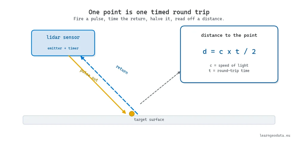
In 1849, Hippolyte Fizeau timed a flash of light out to a mirror five miles across Paris and back, and read off the speed of light.
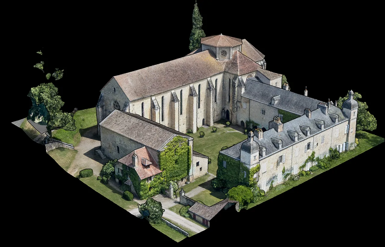
| What it is | The craft of turning raw distance measurements into geometry: read a LAS record, index it, thin it, and separate ground from everything standing on it |
| What you build | A digital terrain model end to end, worked on a 42 million point coastal tile thinned to roughly 6 million points at a 0.25 m voxel |
| Libraries | laspy for LAS and LAZ decoding, Open3D for KDTree and downsampling, PDAL for out-of-core pipelines, NumPy under all three |
| Who it is for | Python engineers meeting scan data for the first time, and anyone whose points keep landing kilometres off site |
| Level | Beginner to intermediate. You need Python and NumPy, no LiDAR background. |
Here is the path this guide takes, so you can jump straight to the part you need:
- What A LiDAR Point Cloud Really Holds
- Reading LAS Files With laspy
- Why One Pulse Returns More Than Once
- Indexing A Cloud For Fast Neighbor Search
- Thinning A Cloud With Voxel Downsampling
- Filtering Ground And Building Terrain Models
- Common Pitfalls In LiDAR Point Cloud Processing
- Where LiDAR Point Cloud Processing Fits
- Build Your First Terrain Model This Week
- Frequently Asked Questions
A LiDAR sensor runs that same experiment backward, a few hundred thousand times a second. It already knows the speed of light. What it measures is the time, and out of that falls a distance to whatever the beam just hit. Every single point in your scan is one of those timed flashes.
So when you open your first .las file and Python hands you a wall of numbers, you are not looking at a picture. You are looking at millions of Fizeau experiments, each one a physical measurement of where a surface sits in space. That is why LiDAR point cloud processing is not image editing. It is the craft of turning raw distance measurements into geometry a machine can actually reason about, and this guide walks you across the whole of it.
What you’ll learn in this article:
- What a LiDAR point actually is, what one LAS record carries beyond XYZ, and why that matters
- How to read a LAS file with laspy and index it with an Open3D KDTree in a handful of lines
- Why a single pulse can return several times, and how to use that
- The cloth simulation settings that decide whether ground extraction succeeds or quietly fails
- The pitfalls that look like corrupt data but are really one forgotten line of code
Estimated reading time: 13 minutes
What A LiDAR Point Cloud Really Holds
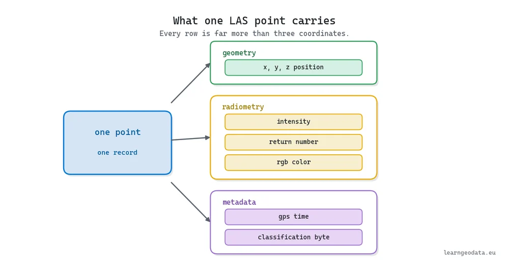
Before you run a single algorithm, ask the plain question: what is actually in this file? A point cloud is a list of XYZ triples, yes, but that is the smallest part of the story. Each row usually carries a stack of extra measurements that turn out to be the difference between a shrug and a real classification.
Intensity tells you how strong the return was, which separates asphalt from grass before you have done any geometry. The return number tells you whether this echo was the first thing the pulse hit or the last. There is a GPS timestamp, sometimes an RGB colour from a fused camera, and a classification byte that a previous processing step may already have filled in.
How you hold all of that in memory quietly sets the ceiling on what feels instant and what makes you go make coffee. Store the cloud as raw points and you keep every measurement, but you have no idea what sits next to what. Drop it into a voxel grid and neighbourhood operations get cheap, but you blur the fine detail. There is no universally correct choice, only the right one for your next operation.
🪐 System Thinking Note: Think of any spatial AI project as three acts: capture, understand, deliver. This whole guide lives in act one, capture, which is roughly a third of the work but sets up the other two thirds. Get the representation and the cleaning right and the understand stage has a fighting chance. Botch it and you will spend the 60 percent of the project that is understanding chasing errors you baked in on day one.
Reading LAS Files With laspy
Airborne and terrestrial scanners hand you LAS files, or their compressed twin, LAZ. Underneath, the bytes follow the ASPRS LAS specification, which pins down the point record formats, the classification codes, and a scaled-integer trick that keeps the files small. You crack it open with laspy, which decodes those bytes into clean NumPy arrays, one per dimension the file stores.
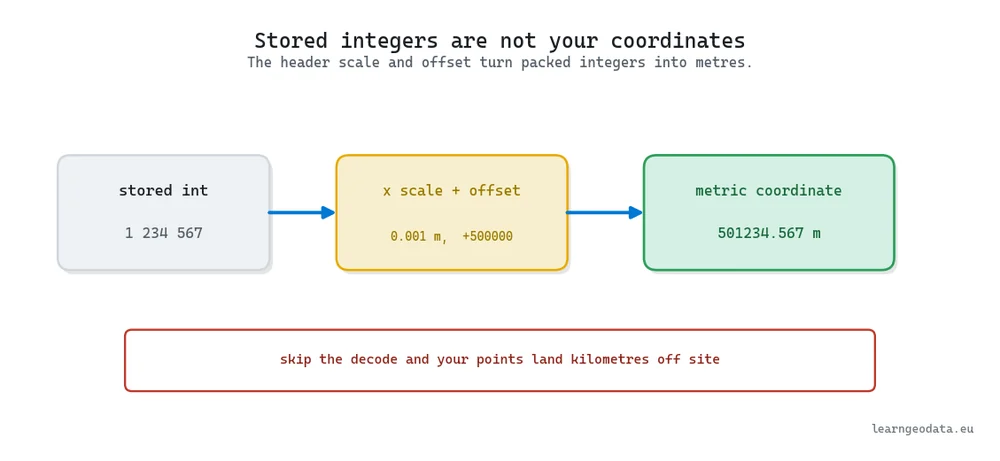
That scaled-integer trick is also the single sharpest trap for a beginner, so it deserves a proper look. To save space, the format never writes your coordinates as floats. It writes small integers, plus a scale and an offset in the header, and you recover the real position by multiplying and adding.
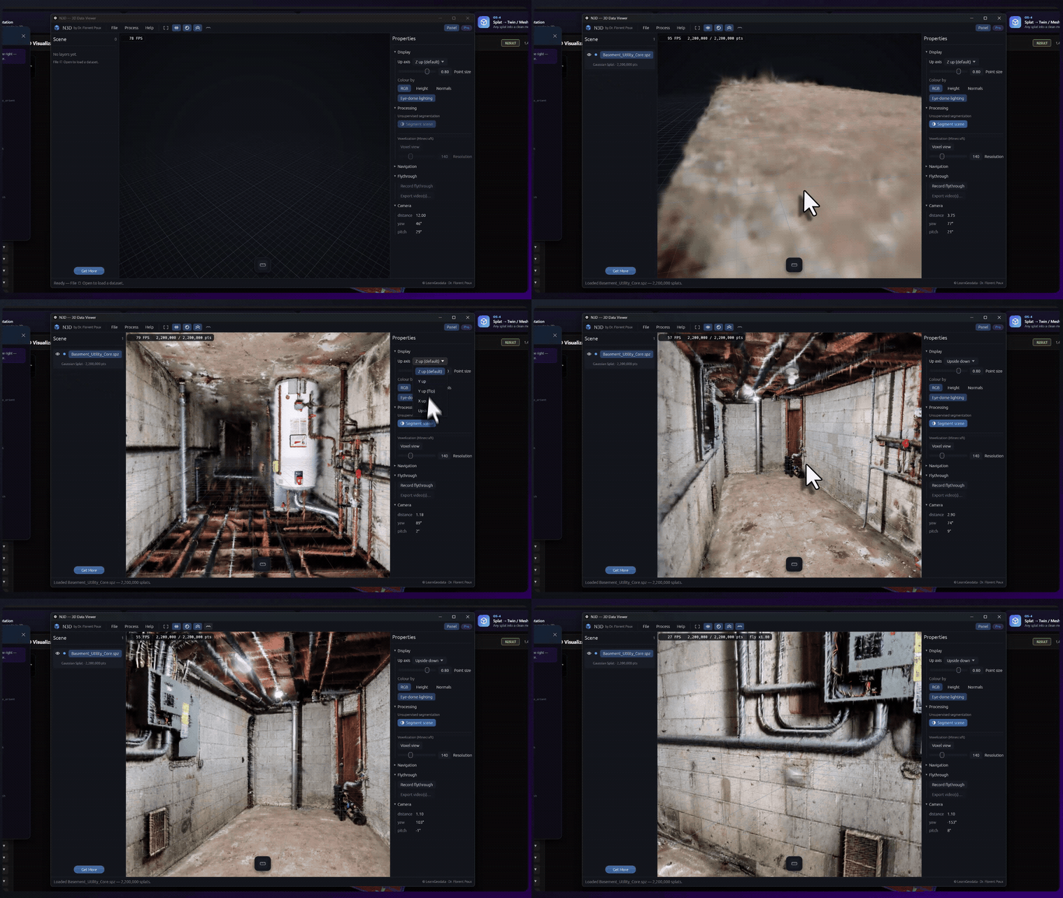
For anything heavier than a single tile, you reach for two more tools, and it helps to know which owns which job. PDAL gives you a stage-based pipeline, written as JSON, that chains reads and filters and writes so you can chew through files far bigger than your RAM. Open3D covers visualization, downsampling, and the neighbourhood queries you are about to meet. With NumPy under all three, that trio reads almost anything you will be handed.
🦚 Florent’s Note: Watch your coordinates on the very first read. laspy applies the decode for you when you call las.x, las.y, las.z, but grab the raw integer dimension by hand and you skip the scale and offset entirely. I have watched a colleague lose an afternoon to a scan that looked broken and was really just sitting 500,000 metres east of where the accessor would have put it. Trust las.x, not the packed field.
Why One Pulse Returns More Than Once
A single laser pulse returns more than once because the beam is not a dimensionless dot. It spreads slightly as it travels, and when it grazes something with gaps in it, a tree is the classic case, part of the beam bounces off the top while the rest keeps going.
So one pulse can hand you several points at different depths. The first return might be the canopy, an intermediate return a branch halfway down, and the last return the bare ground underneath the whole thing.
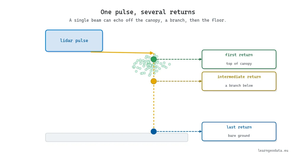
This is not a curiosity, it is a superpower. It is precisely why LiDAR maps terrain under dense vegetation where a camera only ever sees the leaves. And it means the return number field, sitting quietly in every record, is a filter you already own before you compute anything.
🌱 Growing Note: Push this idea one step. Before you run any ground filter, split the cloud by return number: keep only last-or-single returns as your ground candidates and you have thrown out a large slice of the canopy for free, often 30 to 50 percent of the points in a forested tile. The ground filter then has far less to argue with, and it runs faster on the smaller set.
Indexing A Cloud For Fast Neighbor Search
I used to tell people to reach for the fanciest algorithm first. Honestly, that is backwards. The thing that stalls real projects is almost never the algorithm, it is a raw cloud with no notion of what sits near what.
Finding a point’s neighbours in an unindexed cloud means scanning the entire array, every time, and on a big aerial tile that is death by a few million comparisons per query. So the first real move, before ground filtering, before descriptors, before anything, is to give the cloud a spatial index. A KDTree is the workhorse here, and Open3D builds one in a single line.
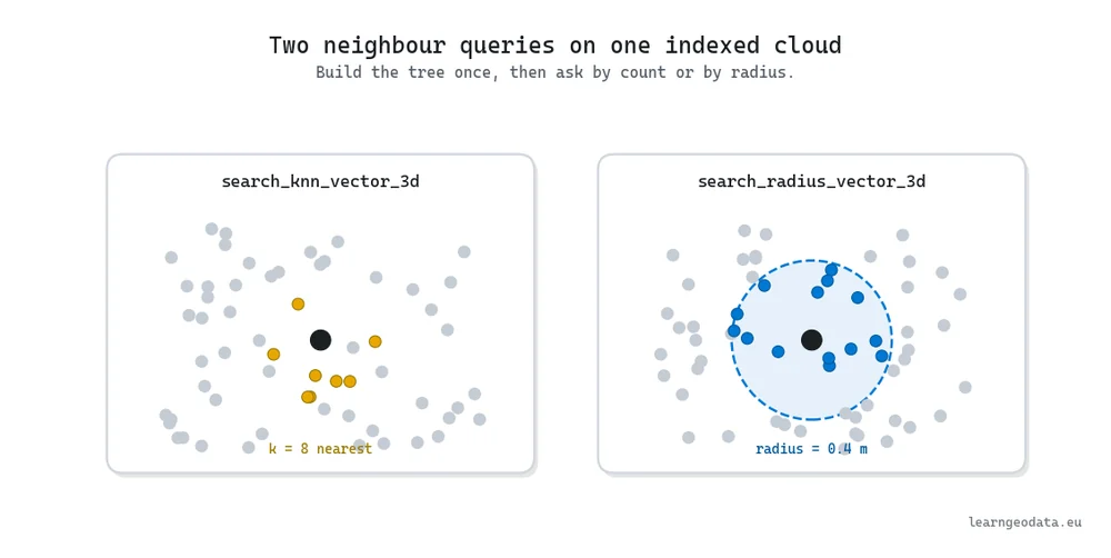
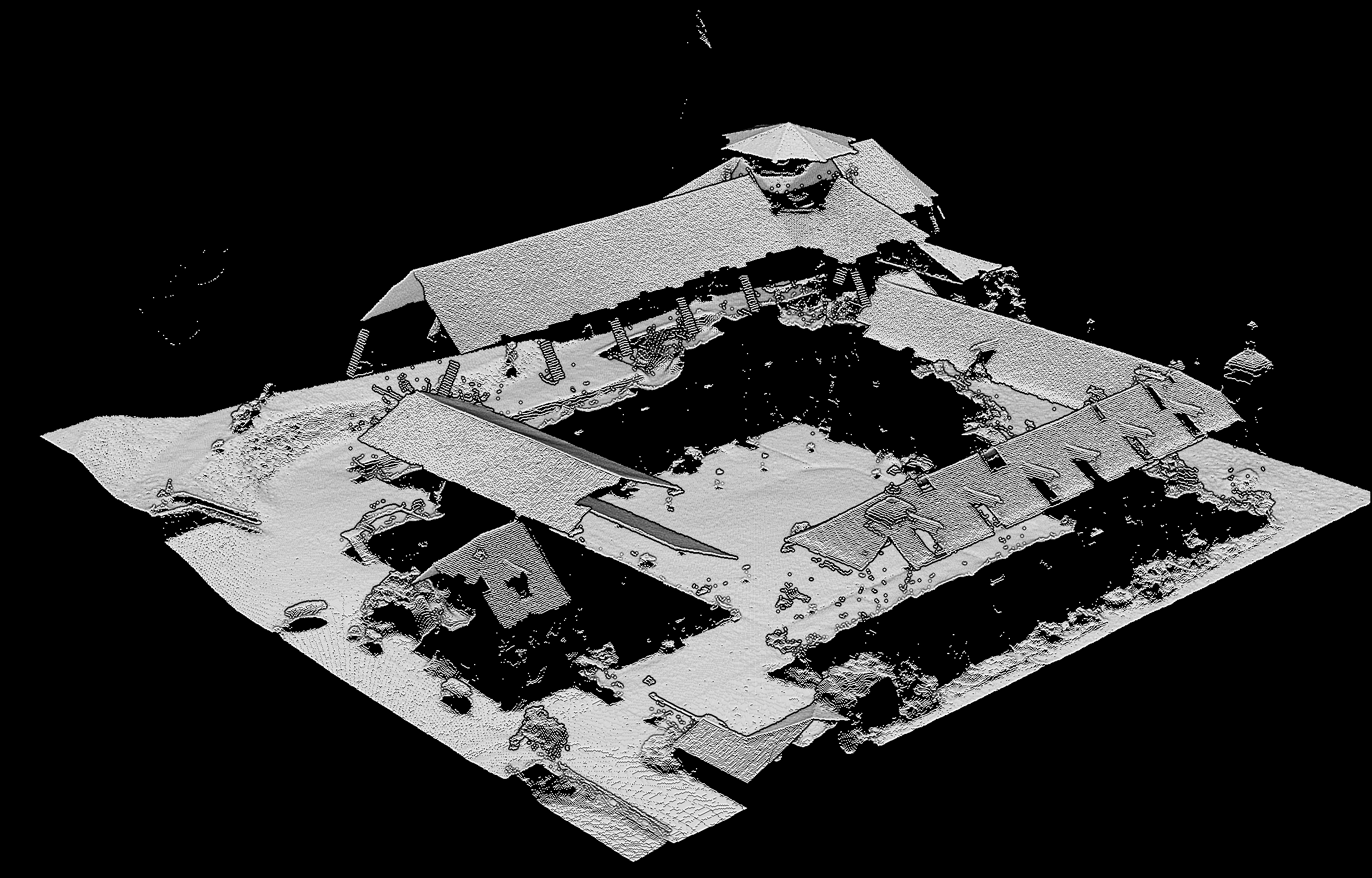
Here is the core loop in real code. laspy pulls the tile into arrays, the coordinates become an Open3D cloud, a voxel grid thins it, and one KDTree makes every later query cheap. Notice there are two query shapes, the k-nearest and the radius search, because you will reach for both depending on whether you want a fixed count or a fixed distance. Those neighbourhoods are the raw material for descriptors, which our point cloud feature extraction guide covers in full.
import laspy
import numpy as np
import open3d as o3d

# laspy applies the header scale and offset, so you get metres, not raw ints
las = laspy.read("riverbank_tile.laz")
xyz = np.column_stack([las.x, las.y, las.z]).astype(np.float64)

# Move the coordinates into an Open3D container
pcd = o3d.geometry.PointCloud()
pcd.points = o3d.utility.Vector3dVector(xyz)

# Thin to one point per 0.20 m cell before anything expensive runs
pcd = pcd.voxel_down_sample(voxel_size=0.20)

# Build the KDTree once, then reuse it for every neighbourhood question
kdtree = o3d.geometry.KDTreeFlann(pcd)
probe = pcd.points[1000]

# k nearest neighbours: the 16 closest points to the probe
k, knn_idx, knn_d2 = kdtree.search_knn_vector_3d(probe, 16)

# radius search: everything within 0.30 m of the probe
n, ball_idx, ball_d2 = kdtree.search_radius_vector_3d(probe, 0.30)
🦥 Geeky Note: Building a KDTree costs about O(N log N) once, and each lookup after that runs in roughly O(log N). On a 42 million point coastal tile, that gap decides whether a 16-nearest search returns in milliseconds or crawls through all 42 million rows on every call. Pay the build cost a single time with KDTreeFlann, then reuse the tree for every descriptor, every filter, every query in the pipeline.
Thinning A Cloud With Voxel Downsampling
A survey tile packs far more points than the later stages actually need. Push all of them through every step and you burn compute you will not get back, so the cheapest speedup in the whole workflow is to thin the cloud up front.
Voxel downsampling is the clean way to do it. You lay an invisible 3D grid over the cloud, and every cell that contains points collapses to one representative point at its centroid. One dial controls the whole thing: the voxel size, in metres.
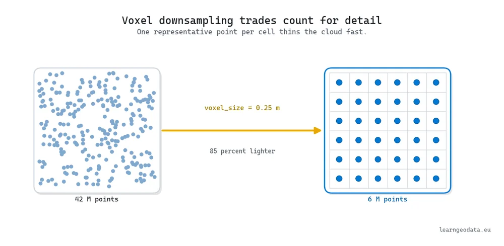
The trade is honest and easy to reason about. A larger cell keeps fewer points and blurs geometry, a smaller cell keeps detail and keeps points. Everything downstream, including the KDTree you just built, runs on the thinned version, so this one choice ripples through every later step. For a deeper look at snapping a cloud onto a grid, see our voxelization tutorial in Python.
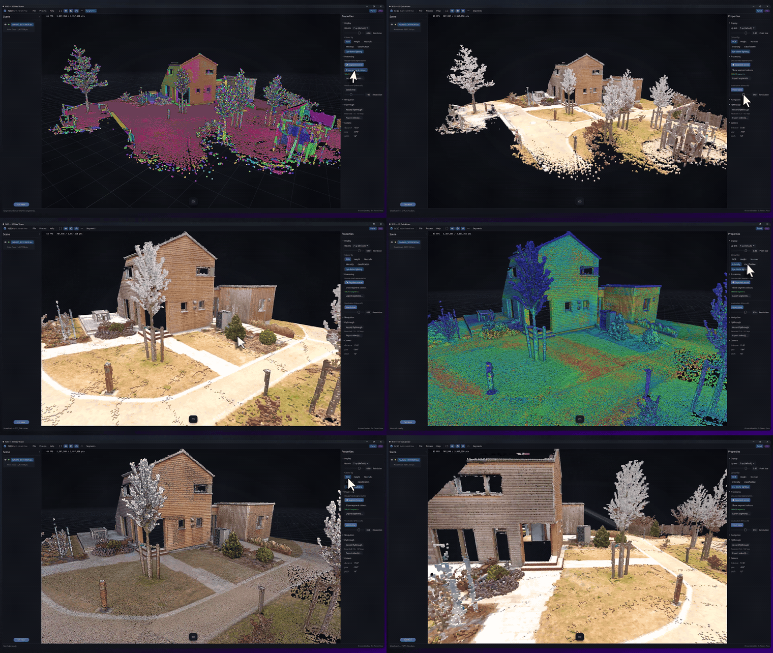
🦚 Florent’s Note: On that 42 million point tile, a 0.25 m voxel took it down to roughly 6 million, an 85 percent cut, and the surfaces that mattered stayed intact. My rule: set the voxel to the smallest feature you genuinely need to keep, not smaller. Terrain work is happy at 0.25 to 0.50 m, while a facade with fine moulding might demand 0.05 m. Guess the value once, look at the result, then commit.
Filtering Ground And Building Terrain Models
Once the cloud is indexed and thinned, the operation that unlocks the rest is pulling the ground away from everything standing on it. Nail it and a whole set of products opens up. Miss it and every product built on top inherits the mistake without ever warning you.
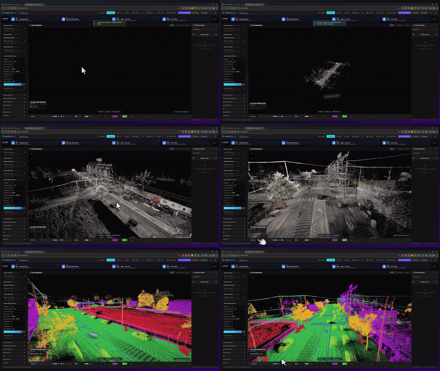
The method I keep returning to is Cloth Simulation Filtering, which Zhang and co-authors published in 2016. Picture something almost tactile: flip the cloud upside down, drape a virtual cloth across the inverted surface, and let gravity settle it into the hollows. The resting cloth traces the terrain, and any point hugging it becomes ground. Few knobs, far kinder to steep slopes than a plain lowest-point grid, and it ships as a ready PDAL filter stage.
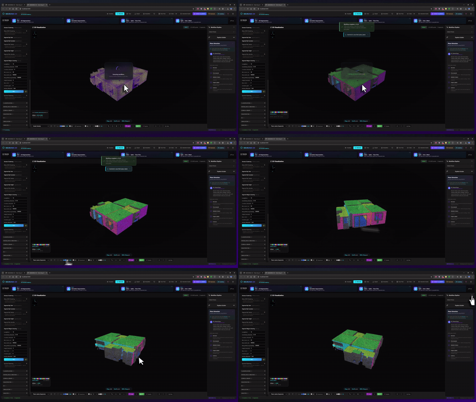
🦥 Geeky Note: CSF lives or dies on three settings. Cloth resolution is the grid spacing, and I run 1.0 m for open coastal terrain. Rigidness is 1 for flat ground, 2 for rolling dunes, 3 for cliffs. The classification threshold, the cloth-to-point distance that counts as ground, sits around 0.45 m here. Set that threshold too tight and a low seawall reads as ground, too loose and the curbs quietly vanish into the terrain.
Everything in that note is a handful of lines of PDAL. A pipeline is a list of stages described as JSON, and you chain them in order: read the tile, settle the cloth, keep only the ground class, then rasterise the result. Because PDAL streams the chain out of core, a tile far larger than your RAM still runs to completion.
import json
import pdal

# A PDAL pipeline is an ordered list of stages, written as JSON.
# Read the tile, label ground with cloth simulation, keep that class,
# then interpolate the ground points straight into a raster DTM.
pipeline = {
    "pipeline": [
        "riverbank_tile.laz",
        {
            "type": "filters.csf",
            "resolution": 1.0,   # cloth grid spacing in metres
            "rigidness": 2,      # 1 flat, 2 rolling, 3 steep terrain
            "threshold": 0.45    # cloth-to-point distance counted as ground
        },
        {
            "type": "filters.range",
            "limits": "Classification[2:2]"   # 2 is the ASPRS ground class
        },
        {
            "type": "writers.gdal",
            "filename": "dtm.tif",
            "resolution": 0.5,    # output raster cell size in metres
            "output_type": "idw"  # inverse-distance fill between ground points
        }
    ]
}

# json.dumps turns the dict into the pipeline string PDAL expects
p = pdal.Pipeline(json.dumps(pipeline))
p.execute()   # runs read -> csf -> range -> gdal, streaming out of core
Once ground is isolated, you interpolate those points onto a regular raster and you have a Digital Terrain Model, the bare earth. Rasterise the highest returns instead and you get a Digital Surface Model, the top of everything. Subtract one from the other and something useful falls out.
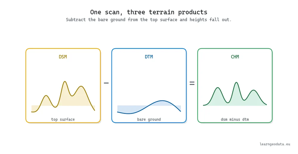
That difference is the trick that makes standing structures far easier to classify. Normalise every point to its height above the ground, and a 4 m tree and a 4 m wall now read as the same height regardless of the slope underneath. A classifier no longer has to untangle terrain shape from object shape, because you already did. Once buildings stand apart from the terrain, turning them into clean city models is the next step, and our guide to vectorising LiDAR into city models shows how.
🌱 Growing Note: Take this one raster further. Rasterise the ground to a 0.5 m DTM, rasterise the first returns to a DSM at the same resolution, and subtract. You now hold a Canopy Height Model you got free from the same scan, and it feeds straight into biomass and forestry estimates. The step up from there is height-normalising the whole cloud before you hand it to a random forest in scikit-learn.
Common Pitfalls In LiDAR Point Cloud Processing
Let me be honest about where this goes wrong, because it rarely fails loudly. LiDAR point cloud processing breaks in quiet ways that look like corrupt data and are usually one small oversight upstream.
Four traps account for a lot of lost afternoons. Reading the raw integer coordinates instead of the decoded ones. Registering scans without setting the source coordinate reference system. Running neighbour queries with no spatial index. And leaving the ground filter on its defaults when your terrain is nothing like the default assumed.
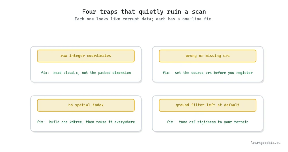
The pattern across all four is the same. A single decision made carelessly early, the coordinate decode, the CRS, the index, the filter parameters, propagates silently and shows up three stages later as a result that is subtly off. That is why you check them at the source, not by staring at the final DTM wondering why it grew a phantom step.
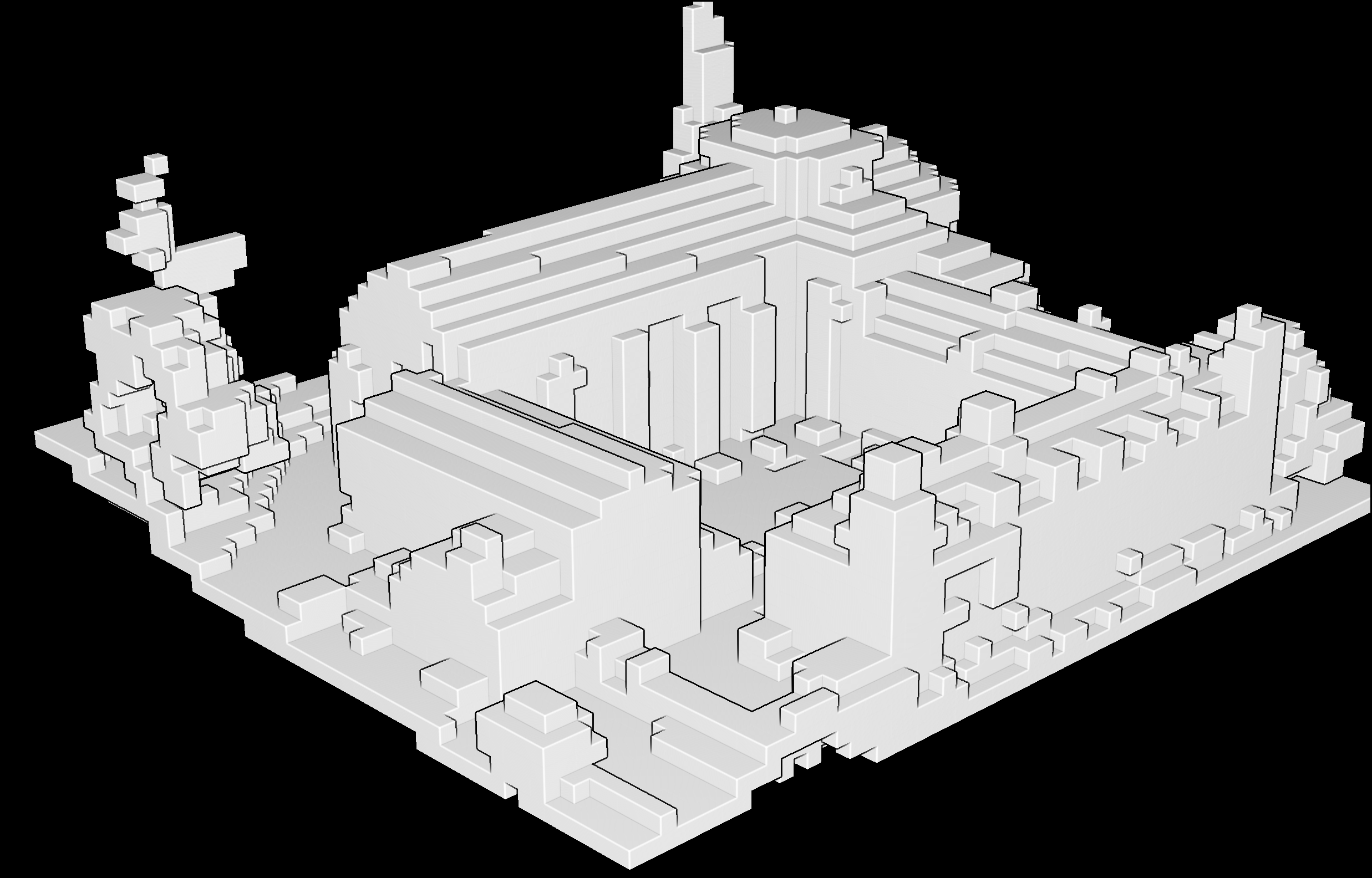
🪐 System Thinking Note: Alignment error does not stay put, it compounds. A 20 cm registration gap between an airborne and a terrestrial scan does more than look wrong: surface normals flip sideways along the seam, ground classification splits into two stacked levels, and your terrain model grows a step nobody put there. Fix the upstream decision first, because every downstream stage inherits it and amplifies it.
Where LiDAR Point Cloud Processing Fits
Processing a scan is one stretch of a longer road, and it helps to see the whole map. This guide covers the capture end, getting reality onto disk, cleaned, aligned, and ready. The stages that follow turn that clean geometry into meaning and then into products someone uses. And when a tile grows too big to open at once, our guide to visualising massive point clouds in Python shows how to stream it.
For the full route, start with the 3D Spatial AI with Python master guide. The closest neighbours are 3D reconstruction in Python (new part, releasing July 22), which builds the same 3D worlds from photographs when you have cameras rather than a scanner, and 3D point cloud segmentation and clustering in Python (new part, releasing July 29), the first understand step once your points are clean. The road then runs into 3D deep learning in Python (new part, releasing August 5), open-vocabulary 3D segmentation in Python (new part, releasing August 12), and point cloud to mesh in Python (new part, releasing August 19).
If you want the guided, hands-on version of everything above with production code beside you, the structured path is the 3D AI program, where I teach the parameter intuition that no single article can hand you.
Build Your First Terrain Model This Week
Reading about this only gets you so far. The understanding sticks the first time you watch a raw scan become a terrain model on your own machine.
So grab one open LAS tile of somewhere you know, a park, a stretch of coast, a campus you walked through. Read it with laspy, voxel-downsample it, build the KDTree, run CSF to pull the ground, and raster a DTM. Then load that terrain into a viewer and hunt for the thing that is wrong, because there is always one: a building that leaked into the ground, a bridge deck the cloth draped straight over, an edge where two tiles disagree.
That single loop, from raw file to flawed-but-real terrain model, teaches you more about where LiDAR genuinely helps and where it quietly misleads than any amount of reading. If you want a soft, free place to start that walk, the free 3D mission is a good first door. And when you are ready to go all the way, from a raw scan to a working spatial AI system, the 3D AI program is where that path is laid out end to end.
So here is the question worth sitting with: when a step in your pipeline drags, do you actually know whether the method is at fault, or whether you locked in the wrong data structure three stages earlier?
Frequently Asked Questions
How Do I Open A LAS File In Python?
Read it with laspy, which decodes the LAS scaled-integer format and returns metric X, Y, Z through the las.x, las.y, las.z accessors, along with intensity, return number, and every other dimension the file stores. The one trap is reaching for the raw integer fields directly, which skips the scale and offset the header holds and lands your points far off site. Stick to the metric accessors and the coordinates come back in true world units.
What Is The Best Library For LiDAR Point Cloud Processing In Python?
There is no single winner, you use a small stack together. Read files with laspy, run heavy out-of-core pipelines with PDAL, and handle visualization plus neighbour queries with Open3D, all sitting on NumPy. That trio reads almost any scan, and the 3D AI program walks through wiring them into one workflow.
How Do I Split Ground From Buildings And Vegetation In A Scan?
Use an automatic ground filter, and Cloth Simulation Filtering is a reliable one, available as a PDAL stage. It settles a virtual cloth against the flipped cloud, treats the points it rests on as terrain, and lets you interpolate those into a raster DTM. Tune the cloth resolution and rigidness to your terrain and the manual cleanup drops to spot fixes rather than whole tiles.
Is Deep Learning Required For LiDAR Processing?
No, and starting there is usually a mistake. For a large share of tasks, hand-designed descriptors with a scikit-learn classifier are enough and stay fully interpretable, so you can see why a point landed in its class. Deep learning earns its keep on subtle classes where descriptors run out of road, and you can grow into that transition through the free 3D mission once your cloud is clean.
How Do I Process A LiDAR Tile That Will Not Fit In RAM?
Stream and tile it with PDAL pipelines, which chain reads, filters, and writes as JSON stages without holding the whole file in memory. You can also downsample early with an Open3D voxel grid, since airborne surveys reach tens of millions of points per tile and thinning up front cuts the count hard while keeping every surface that matters.

