Visualise Massive point cloud in Python.

Tutorial for advanced visualization and interaction with big point cloud data in Python. (Bonus) Learn how to create an interactive segmentation “software”.

Data visualisation is a big enchilada 🌶️: by making a graphical representation of information using visual elements, we can best present and understand trends, outliers, and patterns in data. And you guessed it: with 3D point cloud datasets representing real-world shapes, it is mandatory 🙂.

However, when collected from a laser scanner or 3D reconstruction techniques such as Photogrammetry, point clouds are usually too dense for classical rendering. In many cases, the datasets will far exceed the 10+ million mark, making them impractical for classical visualisation libraries such as Matplotlib.

This means that we often need to go out of our Python script (thus using an I/O function to write our data to a file) and visualise it externally, which can become a super cumbersome process 🤯. I will not lie, that is pretty much what I did the first year of my thesis to try and guess the outcome of specific algorithms🥴.

Would it not be neat to visualise these point clouds directly within your script? Even better, connecting the visual feedback to the script? Imagine, now with the iPhone 12 Pro having a LiDAR; you could create a full online application! Good news, there is a way to accomplish this, without leaving the comfort of your Python Environment and IDE. ☕ and ready?

Step 1: Launch your Python environment.

In the previous article below, we saw how to set up an environment with Anaconda easily and how to use the IDE Spyder to manage your code. I recommend continuing in this fashion if you set yourself up to becoming a fully-fledge python app developer 😆.

Discover 3D Point Cloud Processing with Python
Tutorial to simply set up your python environment, start processing and visualize 3D point cloud data.towardsdatascience.com

If you are using Jupyter Notebook or Google Colab, the script may need some tweaking to make the visualisation back-end work, but deliver unstable performances. If you want to stay on these IDE, I recommend looking at the alternatives to the chosen libraries given in Step 4.

Step 2: Download a point cloud dataset

I illustrated point cloud processing and meshing over a 3D dataset obtained by using photogrammetry and aerial LiDAR from Open Topography in previous tutorials. I will skip the details on LiDAR I/O covered in the article below, and jump right to using the efficient .las file format.

How to automate LiDAR point cloud processing with Python
The ultimate guide on point cloud sub-sampling from scratch, with Python. It covers LiDAR I/O, 3D voxel grid processing…towardsdatascience.com

Only this time, we will use an aerial Drone dataset. It was obtained through photogrammetry making a small DJI Phantom Pro 4 fly on our University campus, gathering some images and running a photogrammetric reconstruction as explained here.

🤓 Note: For this how-to guide, you can use the point cloud in this repository, that I already filtered and translated so that you are in the optimal conditions. If you want to visualize and play with it beforehand without installing anything, you can check out the webGL version.

Step 3: Load the point cloud in the script

We first import necessary libraries within the script (NumPy and LasPy), and load the .las file in a variable called point_cloud.

import numpy as np
import laspy as lp
input_path="D:/CLOUD/POUX/ALL_DATA/"
dataname="2020_Drone_M"
point_cloud=lp.file.File(input_path+dataname+".las", mode="r")

Nice, we are almost ready! What is great, is that the LasPy library also give a structure to the point_cloud variable, and we can use straightforward methods to get, for example, X, Y, Z, Red, Blue and Green fields. Let us do this to separate coordinates from colours, and put them in NumPy arrays:

points = np.vstack((point_cloud.x, point_cloud.y, point_cloud.z)).transpose()
colors = np.vstack((point_cloud.red, point_cloud.green, point_cloud.blue)).transpose()

🤓 Note: We use a vertical stack method from NumPy, and we have to transpose it to get from (n x 3) to a (3 x n) matrix of the point cloud.

Step 4 (Optional): Eventual pre-processing

If your dataset is too heavy, or you feel like you want to experiment on a subsampled version, I encourage you the check out the article below that give you several ways to achieve such a task:

How to automate LiDAR point cloud processing with Python
The ultimate guide on point cloud sub-sampling from scratch, with Python. It covers LiDAR I/O, 3D voxel grid processing…towardsdatascience.com

For convenience, and if you have a point cloud that exceeds 100 million points, we can just quickly slice your dataset using:

factor=10
decimated_points_random = points[::factor]

🤓 Note: Running this will keep 1 row every 10 rows, thus dividing the original point cloud’s size by 10.

Step 5: Choose your visualisation strategy.

Now, let us choose how we want to visualise our point cloud. I will be honest, here: while visualisation alone is great to avoid cumbersome I/O operations, having the ability to include some visual interaction and processing tools within Python is a great addition! Therefore, the solution that I push is using a point cloud processing toolkit that permits exactly this and more. I will still give you alternatives if you want to explore other possibilities ⚖️.

Solution A (Retained): PPTK

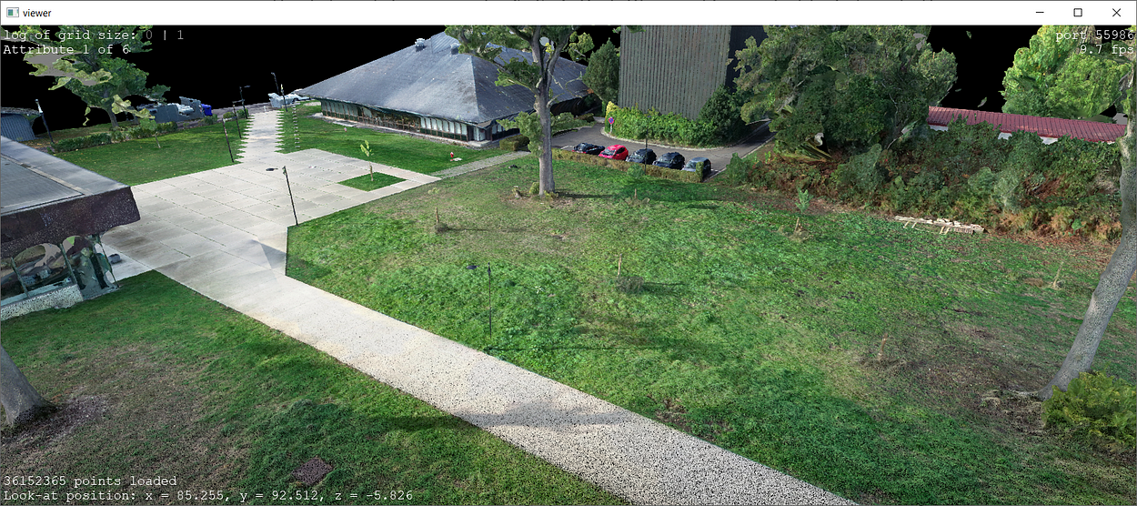
The PPTK package has a 3-d point cloud viewer that directly takes a 3-column NumPy array as input and can interactively visualize 10 to 100 million points. It reduces the number of points that needs rendering in each frame by using an octree to cull points outside the view frustum and to approximate groups of faraway points as single points.

To get started, you can simply install the library using the Pip manager:

pip install pptk

Then you can visualise your previously createdpointsvariable from the point cloud by typing:

import pptk
import numpy as np
v = pptk.viewer(points)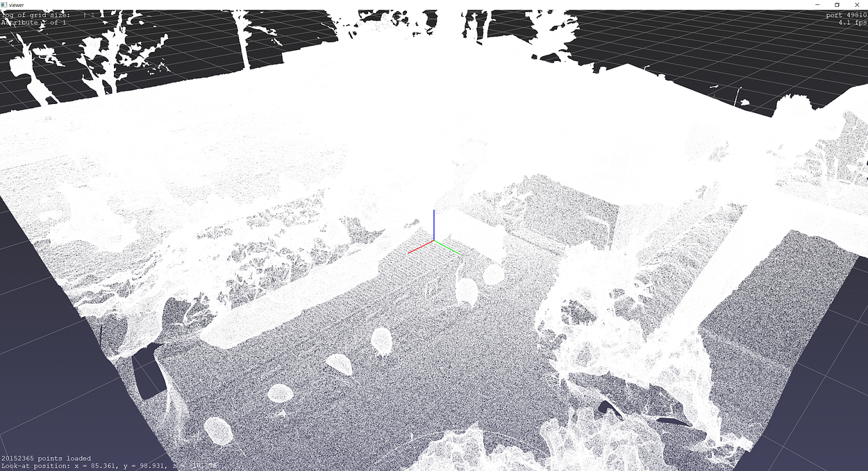

Don’t you think we are missing some colours? Let us solve this by typing in the console:

v.attributes(colors/65535)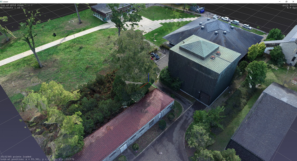

🤓 Note: Our colour values are coded on 16bits from the .las file. We need the values in a [0,1] interval; thus, we divide by 65535.

That is way better! But what if we also want to visualise additional attributes? Well, you just link your attributes to your path, and it will update on the fly.

💡 Hint: Do not maximize the size of the window to keep a nice framerate over 30 FPS. The goal is to have the best execution runtime while having a readable script

You can also parameterize your window to show each attributes regarding a certain colour ramp, managing the point size, putting the background black and not displaying the grid and axis information:

v.color_map('cool')
v.set(point_size=0.001,bg_color=[0,0,0,0],show_axis=0,show_grid=0)

Alternative B: Open3D

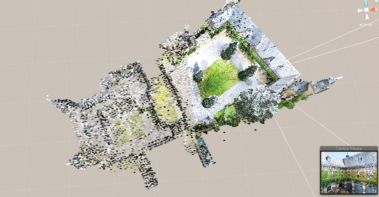
For anybody wondering for an excellent alternative to read and display point clouds in Python, I recommend Open3D. You can use the Pip package manager as well to install the necessary library:

pip install open3d

We already used Open3d in the tutorial below, if you want to extend your knowledge on 3D meshing operations:

5-Step Guide to generate 3D meshes from point clouds with Python
Tutorial to generate 3D meshes (.obj, .ply, .stl, .gltf) automatically from 3D point clouds using python. (Bonus)…towardsdatascience.com

This will install Open3D on your machine, and you will then be able to read and display your point clouds by executing the following script:

import open3d as o3d

pcd = o3d.geometry.PointCloud()
pcd.points = o3d.utility.Vector3dVector(points)
pcd.colors = o3d.utility.Vector3dVector(colors/65535)
pcd.normals = o3d.utility.Vector3dVector(normals)

o3d.visualization.draw_geometries([pcd])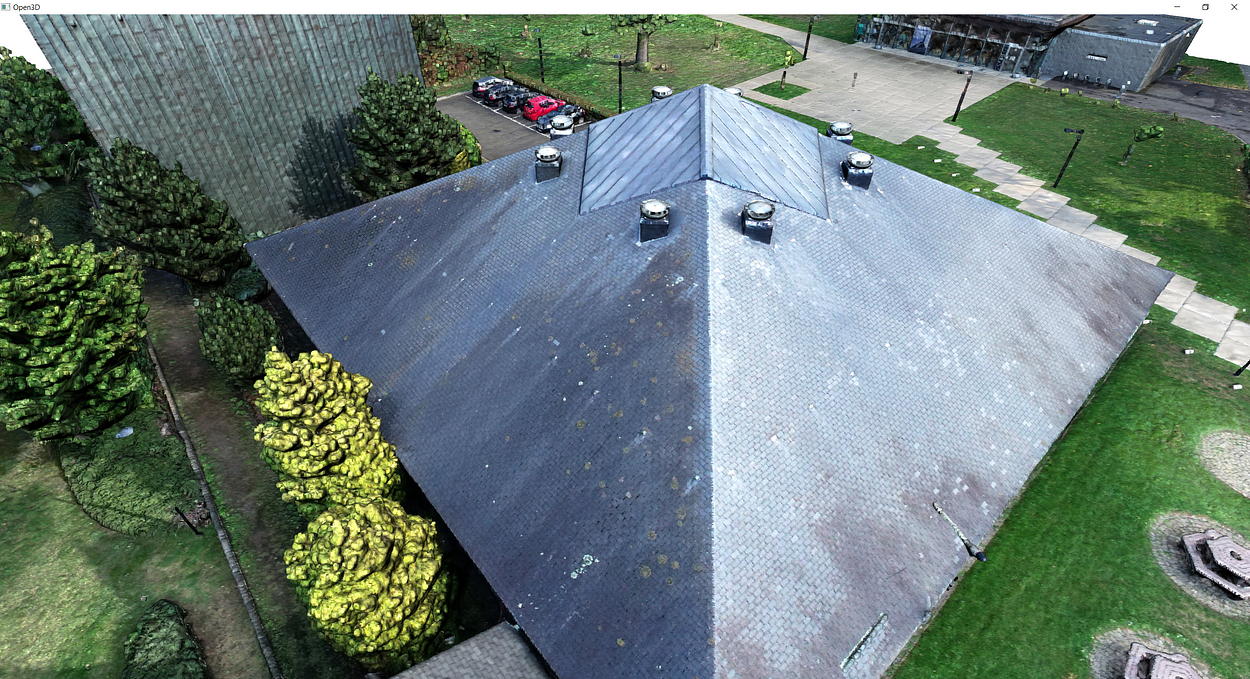

Open3D is actually growing, and you can have some fun ways to display your point cloud to fill eventual holes like creating a voxel structure:

voxel_grid = o3d.geometry.VoxelGrid.
create_from_point_cloud(pcd,voxel_size=0.40)

o3d.visualization.draw_geometries([voxel_grid])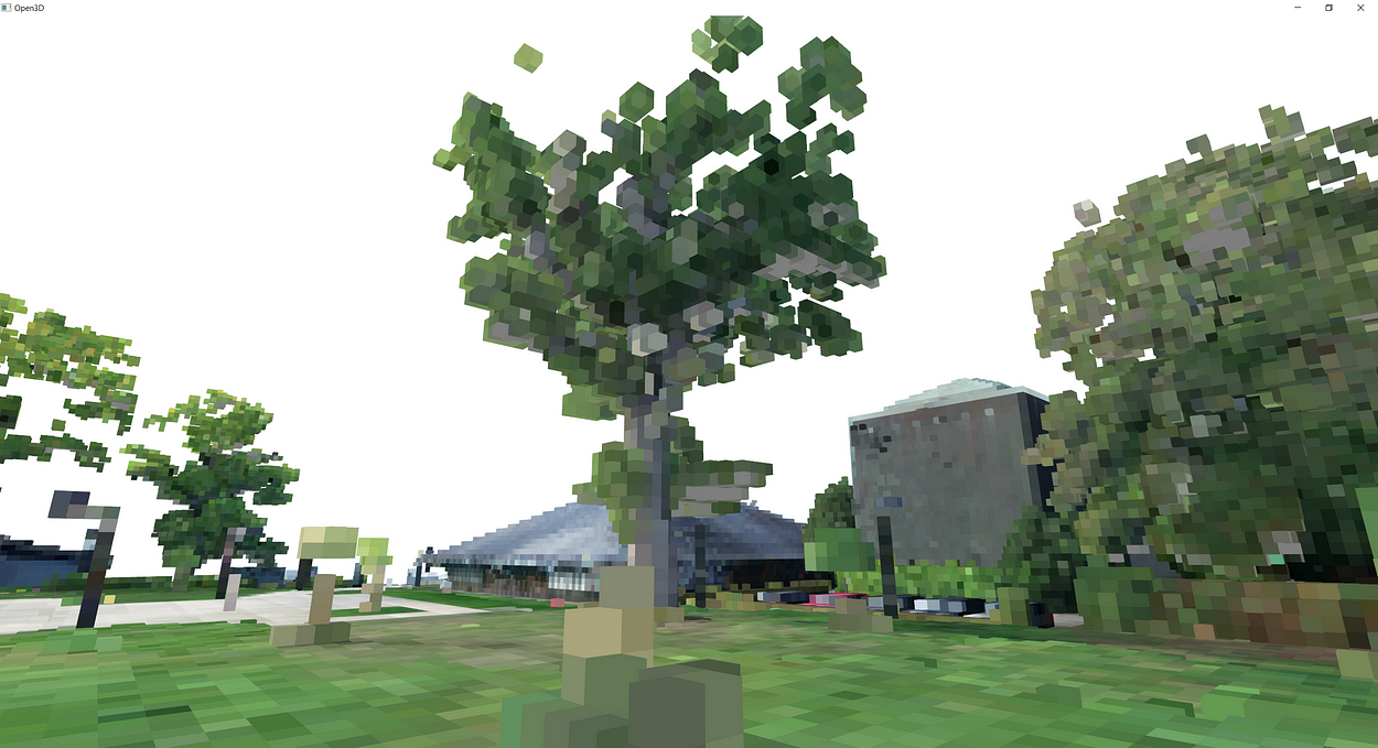

🤓 Note: Why is Open3d not the choice at this point? If you work with datasets under 50 million points, then it is what I would recommend. If you need to have interactive visualization above this threshold, I recommend either sampling the dataset for visual purposes, or using PPTK which is more efficient for visualizing as you have the octree structure created for this purpose.

Other (Colab-friendly) alternatives: Pyntcloud and Pypotree

If you would like to enable simple and interactive exploration of point cloud data, regardless of which sensor was used to generate it or what the use case is, I suggest you look into Pyntcloud, or PyPotree. These will allow you to visualise the point cloud in your notebook, but beware of the performances! Pyntcloud actually rely on Matplotlib, and PyPotree demands I/O operations; thus, both are actually not super-efficient. Nevertheless, I wanted to mention them because for small point clouds and simple experiment in Google Colab, you can integrate the visualisation. Some examples:

### PyntCloud ###
conda install pyntcloud -c conda-forge
from pyntcloud import PyntCloud

pointcloud = PyntCloud.from_file("example.ply")
pointcloud.plot()

### PyntCloud ###
pip install pypotree

import pypotree 
import numpy as np
xyz = np.random.random((100000,3))
cloudpath = pypotree.generate_cloud_for_display(xyz)
pypotree.display_cloud_colab(cloudpath)

Step 6: Interact with the point cloud

Back to PPTK. To make an interactive selection, say the car on the parking lot, I will move my camera top view (shortcut is 7), and I will make a selection dragging a rectangle selection holding Ctrl+LMB.

💡 Hint: If you are unhappy with the selection, a simple RMB will erase your current selection(s). Yes, you can make multiple selections 😀.

Once the selection is made, you can return to your Python Console and then get the assignment’s point identifiers.

selection=v.get('selected')

This will actually returns a 1D array like this:

You can actually extend the process to select more than one element at once (Ctrl+LMB) while refining the selection removing specific points (Ctrl+Shift+LMB ).

After this, it becomes effortless to apply a bunch of processes interactively over your selection variable that holds the index of selected points.

Let us replicate a scenario where you automatically refine your initial selection (the car) between ground and non-ground elements.

Step 7: Towards an automatic segmentation

In the viewer that contain the full point cloud, stored in the variable v, I make the following selection selection=v.get('selected') :

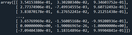
Then I compute normals for each points. For this, I want to illustrate another key takeaway of using PPTK: The function estimate_normals, which can be used to get a normal for each point based on either a radius search or the k-nearest neighbours. Don’t worry, I will illustrate in-depth these concepts in another guide, but for now, I will run it by using the 6 nearest neighbours to estimate my normals:

normals=pptk.estimate_normals(points[selection],k=6,r=np.inf)

💡 Hint: Remember that the selection variable holds the indexes of the points, i.e. the “line number” in our point cloud, starting at 0. Thus, if I want to work only on this point subset, I will pass it as points[selection] . Then, I choose the k-NN method using only the 6 nearest neighbours for each point, by also setting the radius parameter to np.inf which make sure I don’t use it. I could also use both constraints, or set k to -1 if I want to do a pure radius search.

This will basically return this:

Then, I want to filter AND return the original points’ indexes that have a normal not colinear to the Z-axis. I propose to use the following line of code:

idx_normals=np.where(abs(normals[...,2])<0.9)

🤓 Note: The normals[...,2], is a NumPy way of saying that I work only on the 3rd column of my 3 x n point matrix, holding the Z attribute of the normals. It is equivalent to normals[:,2]. Then, I take the absolute value as the comparing point because my normals are not oriented (thus can point toward the sky or towards the earth centre), and will only keep the one that answer the condition <0.9, using the function np.where().

To visualise the results, I create a new viewer window object:

viewer1=pptk.viewer(points[idx_normals],colors[idx_normals]/65535)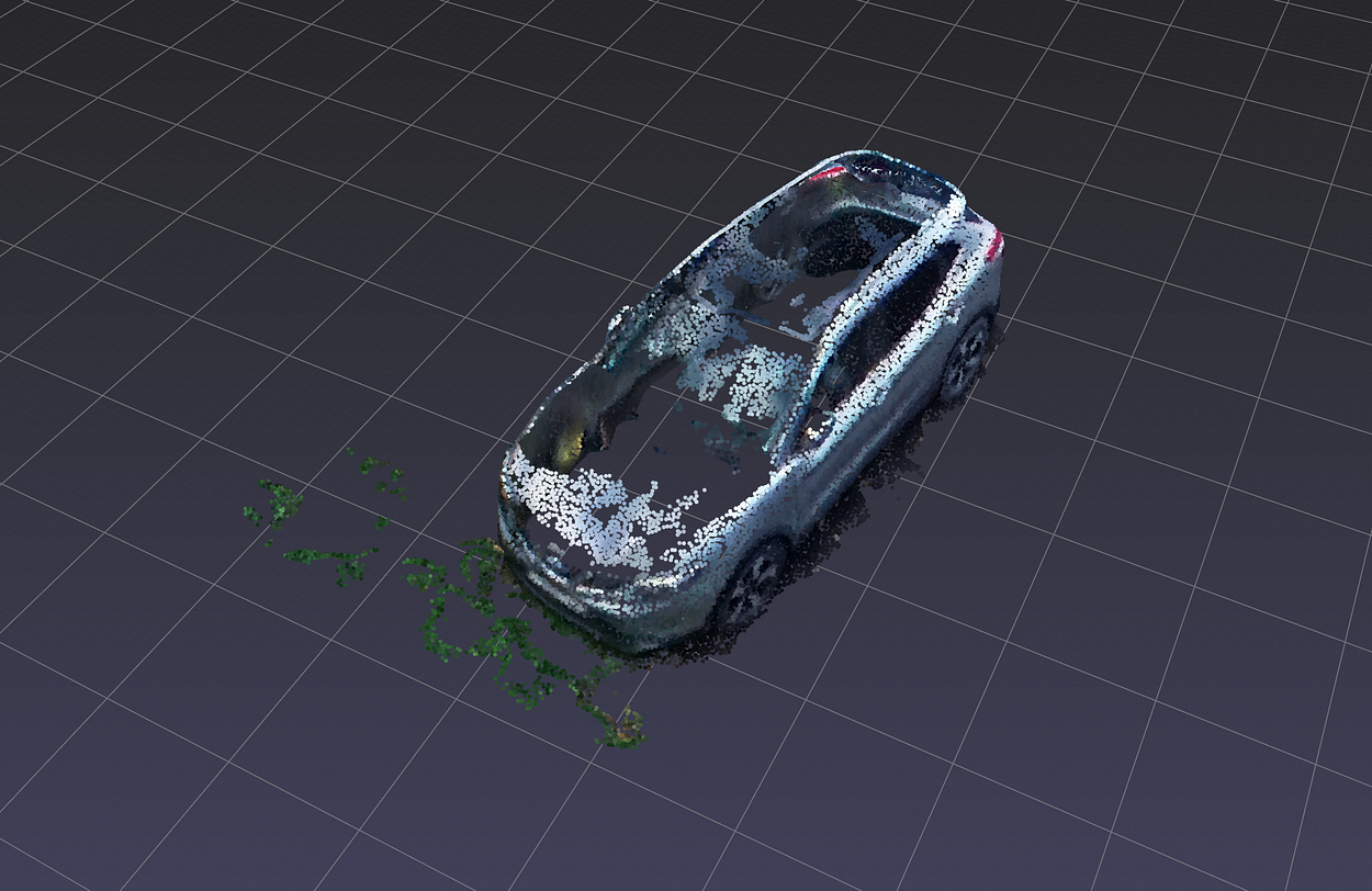

As you can see, we also filtered some points part of the car. This is not good 🤨. Thus, we should combine the filtering with another filter that makes sure only the points close to the ground are chosen as host of the normals filtering:

idx_ground=np.where(points[...,2]>np.min(points[...,2]+0.3))
idx_wronglyfiltered=np.setdiff1d(idx_ground, idx_normals)
idx_retained=np.append(idx_normals, idx_wronglyfiltered)

viewer2=pptk.viewer(points[idx_retained],colors[idx_retained]/65535)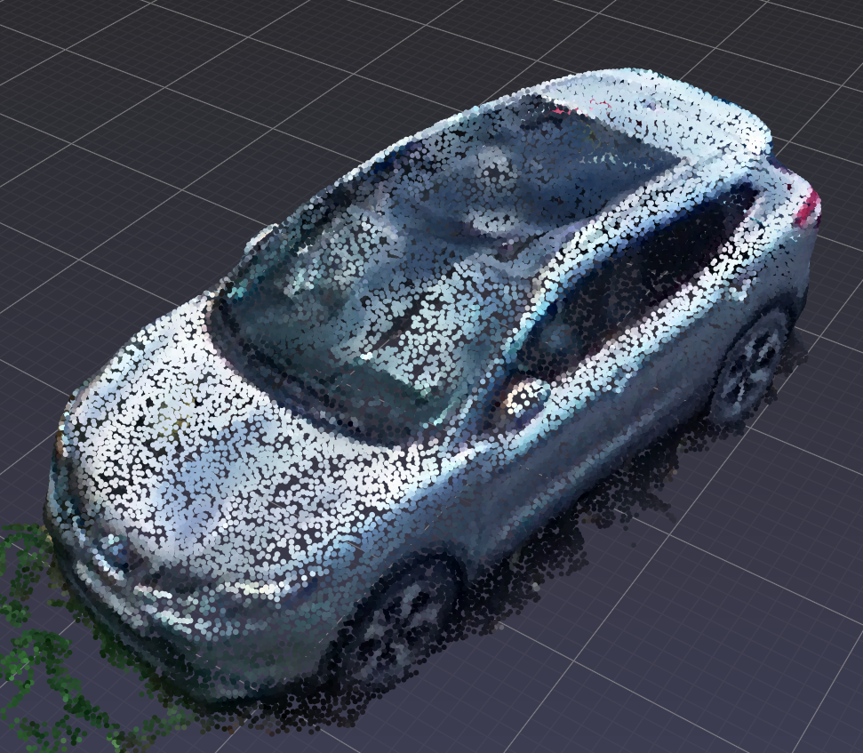

This is nice! And now, you can just explore this powerful way of thinking and combine any filtering (for example playing on the RGB to get away with the remaining grass …) to create a fully interactive segmentation application. Even better, you can combine it with 3D Deep Learning Classification! Ho-ho! But that is for another time 😉.

Step 8: Package your script with functions

Finally, I suggest packaging your script into functions so that you can directly reuse part of it as blocks. We can first define a preparedata(), that will take as input any .laspoint cloud, and format it :

def preparedata():
    input_path="D:/CLOUD/OneDrive/ALL_DATA/GEODATA-ACADEMY/"
    dataname="2020_Drone_M_Features"
    point_cloud=lp.file.File(input_path+dataname+".las", mode="r")
    points = np.vstack((point_cloud.x, point_cloud.y, point_cloud.z) 
    ).transpose()
    colors = np.vstack((point_cloud.red, point_cloud.green,
    point_cloud.blue)).transpose()
    normals = np.vstack((point_cloud.normalx, point_cloud.normaly, 
    point_cloud.normalz)).transpose()
    return point_cloud,points,colors,normals

Then, we write a display function pptkviz, that return a viewer object:

def pptkviz(points,colors):
    v = pptk.viewer(points)
    v.attributes(colors/65535)
    v.set(point_size=0.001,bg_color= [0,0,0,0],show_axis=0,
    show_grid=0)
    return v

Additionally, and as a bonus, here is the function cameraSelector, to get the current parameters of your camera from the opened viewer:

def cameraSelector(v):
    camera=[]
    camera.append(v.get('eye'))
    camera.append(v.get('phi'))
    camera.append(v.get('theta'))
    camera.append(v.get('r'))
    return np.concatenate(camera).tolist()

And we define the computePCFeatures function to automate the refinement of your interactive segmentation:

def computePCFeatures(points, colors, knn=10, radius=np.inf):
    normals=pptk.estimate_normals(points,knn,radius)
    idx_ground=np.where(points[...,2]>np.min(points[...,2]+0.3))
    idx_normals=np.where(abs(normals[...,2])<0.9)
    idx_wronglyfiltered=np.setdiff1d(idx_ground, idx_normals)
    common_filtering=np.append(idx_normals, idx_wronglyfiltered)
    return points[common_filtering],colors[common_filtering]

Et voilà 😁, you now just need to launch your script containing the functions above and start interacting on your selections using computePCFeatures, cameraSelector, and more of your creations:

import numpy as np
import laspy as lp
import pptk

#Declare all your functions here

if __name__ == "__main__":
    point_cloud,points,colors,normals=preparedata()
    viewer1=pptkviz(points,colors,normals)

It is then easy to call the script and then use the console as the bench for your experiments. For example, I could save several camera positions and create an animation:

cam1=cameraSelector(v)
#Change your viewpoint then -->
cam2=cameraSelector(v)
#Change your viewpoint then -->
cam3=cameraSelector(v)
#Change your viewpoint then -->
cam4=cameraSelector(v)

poses = []
poses.append(cam1)
poses.append(cam2)
poses.append(cam3)
poses.append(cam4)
v.play(poses, 2 * np.arange(4), repeat=True, interp='linear')

Conclusion

You just learned how to import, visualize and segment a point cloud composed of 30+ million points! Well done! Interestingly, the interactive selection of point cloud fragments and individual points performed directly on GPU can now be used for point cloud editing and segmentation in real-time. But the path does not end here, and future posts will dive deeper into point cloud spatial analysis, file formats, data structures, segmentation [2–4], animation and deep learning [1]. We will especially look into how to manage big point cloud data as defined in the article below.

The Future of 3D Point Clouds: a new perspective
Discrete spatial datasets known as point clouds often lay the groundwork for decision-making applications. But can they…towardsdatascience.com

My contributions aim to condense actionable information so you can start from scratch to build 3D automation systems for your projects. You can get started today by taking a formation at the Geodata Academy.

References

1. Poux, F., & J.-J Ponciano. (2020). Self-Learning Ontology For Instance Segmentation Of 3d Indoor Point Cloud. ISPRS Int. Arch. of Pho. & Rem. XLIII-B2, 309–316; https://doi.org/10.5194/isprs-archives-XLIII-B2–2020–309–2020

2. Poux, F., & Billen, R. (2019). Voxel-based 3D point cloud semantic segmentation: unsupervised geometric and relationship featuring vs deep learning methods. ISPRS International Journal of Geo-Information. 8(5), 213; https://doi.org/10.3390/ijgi8050213

3. Poux, F., Neuville, R., Nys, G.-A., & Billen, R. (2018). 3D Point Cloud Semantic Modelling: Integrated Framework for Indoor Spaces and Furniture. Remote Sensing, 10(9), 1412. https://doi.org/10.3390/rs10091412

4. Poux, F., Neuville, R., Van Wersch, L., Nys, G.-A., & Billen, R. (2017). 3D Point Clouds in Archaeology: Advances in Acquisition, Processing and Knowledge Integration Applied to Quasi-Planar Objects. Geosciences, 7(4), 96. https://doi.org/10.3390/GEOSCIENCES7040096

Originally published in Towards Data Science.