Learn 3D point cloud segmentation with Python

Learn 3D point cloud segmentation with Python

A complete python tutorial to automate point cloud segmentation and 3D shape detection using multi-order RANSAC and unsupervised clustering (DBSCAN).

If you have worked with point clouds in the past (or, for this matter, with data), you know how important it is to find patterns between your observations 📈. Indeed, we often need to extract some higher-level knowledge that heavily relies on determining “objects” formed by data points that share a pattern.

This is a task that is accomplished quite comfortably by our visual cognitive system. However, mimicking this human capability by computational methods is a highly challenging problem 🤯. Basically, we want to leverage the predisposition of the human visual system to group sets of elements.

But why is point cloud segmentation useful?

Excellent question! Actually, the cardinal motivations for point cloud segmentation are threefold:

• Firstly, it provides end-users with the flexibility to efficiently access and manipulates individual content through higher-level generalisations: segments.
• Secondly, it creates a compact representation of the data wherein all subsequent processing can be done at a regional level instead of the individual point level, resulting in potentially significant computational gains.
• Finally, it gives the ability to extract relationships between neighbourhoods, graphs and topology, which is non-existent in raw point-based data sets.

For these reasons, segmentation is predominantly employed as a pre-processing step to annotate, enhance, analyse, classify, categorise, extract and abstract information from point cloud data. But the real question now. How do we do it?

Aaand… let’s open the box 👐!

Quick point cloud segmentation theory with 2 key concepts

In this tutorial, I already made a selection for you of two of the best and more robust approaches that you will master at the end. We will rely on two central and efficient approaches: RANSAC and Euclidean Clustering through DBSCAN. But before using them, it is, I guess 😀, Important to understand the main idea, simply put.

RANSAC

So RANSAC stands for RANdom SAmple Consensus, and it is a quite simple but highly effective algorithm that you can use if your data is affected by outliers, which is our case 😊. Indeed, whenever you work with real-world sensors, your data will never be perfect. And quite often, your sensor data is affected by outliers. And RANSAC is a kind of a trial-and-error approach that will group your data points into two segments: an inlier set and an outlier set. Then, you can forget about the outliers and work with your inliers.

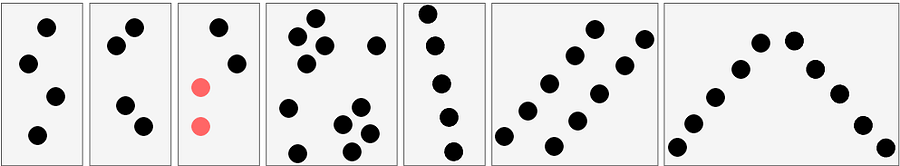
So let me use a tiny but simple example to illustrate how RANSAC works. Let us say that we want to fit a plane through the point cloud below. How can we do that?

First, we create a plane from the data, and for this, we randomly select 3 points from the point cloud necessary to establish a plane. And then, we simply check how many of the remaining points kind of fall on the plane (to a certain threshold), which will give a score to the proposal.

Then, we repeat the process with 3 new random points and see how we are doing. Is it better? Is it worse? And again, we repeat this process over and over again, let’s say 10 times, 100 times, 1000 times, and then we select the plane model which has the highest score (i.e. which has the best “support” of the remaining data points). And that will be our solution: the supporting points plus the three points that we have sampled constitute our inlier point set, and the rest is our outlier point set. Easy enough, hun 😁?

Haha, but for the sceptics, don’t you have a rising question? How do we actually determine how many times we should repeat the process? How often should we try that? Well, that is actually something that we can compute, but let put it aside for now to focus on the matter at hand: point cloud segmentation 😉.

Euclidean Clustering (DBSCAN)

With point cloud datasets, we often need to group sets of points spatially contiguous, as illustrated below. But how can we do this efficiently?

The DBSCAN (Density-Based Spatial Clustering of Applications with Noise) algorithm was introduced in 1996 for this purpose. This algorithm is widely used, which is why it was awarded a scientific contribution award in 2014 that has stood the test of time.

DBSCAN iterates over the points in the dataset. For each point that it analyzes, it constructs the set of points reachable by density from this point: it computes the neighbourhood of this point, and if this neighbourhood contains more than a certain amount of points, it is included in the region. Each neighbouring points go through the same process until it can no longer expand the cluster. If the point considered is not an interior point, i.e. it does not have enough neighbours, it will be labelled as noise. This allows DBSCAN to be robust to outliers since this mechanism isolates them. How cool is that 😆?

Ah, I almost forgot. The choice of parameters (ϵ for the neighbourhood and n_min for the minimal number of points) can also be tricky: One must take great care when setting parameters to create enough interior points (which will not happen if n_min is too large or ϵ too small). In particular, this means that DBSCAN will have trouble finding clusters of different densities. BUT, DBSCAN has the great advantage of being computationally efficient without requiring to predefine the number of clusters, unlike Kmeans, for example. Finally, it allows finding clusters of arbitrary shape.

And now, let us put all of this mumbo jumbo into a super useful “software” through a 5-Step process 💻!

Step 1: The (point cloud) data, always the data 😁

In previous tutorials, I illustrated point cloud processing and meshing over a 3D dataset obtained by using photogrammetry and aerial LiDAR from Open Topography. This time, we will use a dataset that I gathered using a Terrestrial Laser Scanner!

I will skip the details on I/O operations and file formats but know that they are covered in the articles below if you want to clarify or build fully-fledged expertise 🧐. Today, we will jump right to using the well known .ply file format.

How to automate LiDAR point cloud processing with Python
The ultimate guide on point cloud sub-sampling from scratch, with Python. It covers LiDAR I/O, 3D voxel grid processing…towardsdatascience.com

5-Step Guide to generate 3D meshes from point clouds with Python
Tutorial to generate 3D meshes (.obj, .ply, .stl, .gltf) automatically from 3D point clouds using python. (Bonus)…towardsdatascience.com

🤓 Note: For this how-to guide, you can use the point cloud in this repository, that I already filtered and translated so that you are in the optimal conditions. If you want to visualize and play with it beforehand without installing anything, you can check out the webGL version.

Step 2: Set up your Python environment.

In the previous article below, we saw how to set up an environment with Anaconda easily and how to use the IDE Spyder to manage your code. I recommend continuing in this fashion if you set yourself up to becoming a fully-fledged python app developer 😆.

Discover 3D Point Cloud Processing with Python
Tutorial to simply set up your python environment, start processing and visualize 3D point cloud data.towardsdatascience.com

But hey, if you prefer to do everything from scratch in the next 5 minutes, I also give you access to a Google Colab notebook that you will find at the end of the article. There is nothing to install; you can just save it to your google drive and start working with it, also using the free datasets from Step 1☝️.

🤓 Note: I highly recommend using a desktop IDE such as Spyder and avoiding Google Colab or Jupyter IF you need to visualise 3D point clouds using the libraries provided, as they will be unstable at best or not working at worse (unfortunately…).

Step 3: First Segmentation Round

Well, for quickly getting results, I will take a “parti-pris”. Indeed, we will accomplish a nice segmentation by following a minimalistic approach to coding 💻. That means being very picky about the underlying libraries! We will use three very robust ones, namely numpy, matplotlib, and open3d.

Okay, to install the library package above in your environment, I suggest you run the following command from the terminal (also, notice the open3d-admin channel):

conda install numpy
conda install matplotlib
conda install -c open3d-admin open3d

🤓 Disclaimer Note: We choose Python, not C++ or Julia, so performances are what they are 😄. Hopefully, it will be enough for your application 😉, for what we call “offline” processes (not real-time).

And it is the long-awaited time now to get to see the first results!

How to implement RANSAC over 3D point clouds?

The basics

Let us first import the data in the pcd variable, with the following line:

pcd = o3d.io.read_point_cloud("your_path/kitchen.ply")

Do you want to do wonders quickly? Well, I have excellent news, open3d comes equipped with a RANSAC implementation for planar shape detection in point clouds. The only line to write is the following:

plane_model, inliers = pcd.segment_plane(distance_threshold=0.01, ransac_n=3, num_iterations=1000)

🤓 Note: As you can see, the segment_plane() method holds 3 parameters. These are the distance threshold (distance_threshold) from the plane to consider a point inlier or outlier, the number of sampled points drawn (3 here, as we want a plane) to estimate each plane candidate (ransac_n) and the number of iterations (num_iterations). These are standard values, but beware that depending on the dataset at hand, the distance_threshold should be double-checked.

Inliers vs Outliers

The result of the line above is the best plane candidate parameters a,b,c and d captured in plane_model, and the index of the points that are considered as inliers, captured in inliers.

Let us now visualize the results, shall we? For this, we actually have to select the points based on the indexes captured in inliers, and optionally select all the others as outliers. How do we do this? Well, like this:

inlier_cloud = pcd.select_by_index(inliers)
outlier_cloud = pcd.select_by_index(inliers, invert=True)

🤓 Note: The argument invert=True permits to select the opposite of the first argument, which means all indexes not present in inliers.

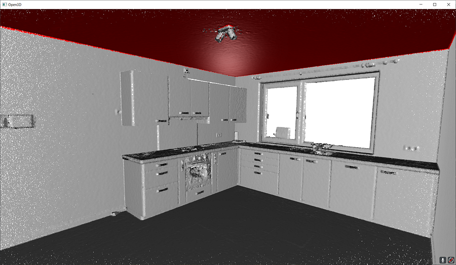
Okay, now your variables hold the points, but before visualizing the results, I propose that we paint the inliers in red and the rest grey. For this, you can just pass a list of R, G, B values as floats like this:

inlier_cloud.paint_uniform_color([1, 0, 0])
outlier_cloud.paint_uniform_color([0.6, 0.6, 0.6])

And now, let us visualise the results with the following line:

o3d.visualization.draw_geometries([inlier_cloud, outlier_cloud])

🤓 Note: If you want to grasp better the geometry washed up by the colour, you can compute normals using the following command beforehand: pcd.estimate_normals(search_param=o3d.geometry.KDTreeSearchParamHybrid(radius=0.1, max_nn=16), fast_normal_computation=True). This will make sure you get a much nicer rendering, as below😉.

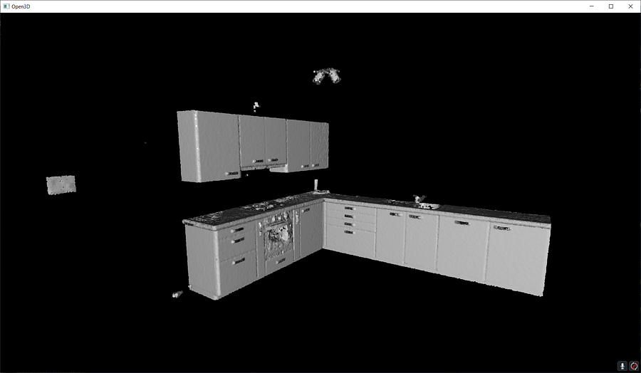
Great! You know how to segment your point cloud in an inlier point set and an outlier point set 🥳! Now, let us study how to find some clusters close to one another. So let us imagine that once we detected the big planar portions, we have some “floating” objects that we want to delineate. How to do this? (yes, it is a false question, I have the answer for you 😀)

How to use DBSCAN over point clouds?

The basics

First, we select a sample, where we assume we got rid of all the planar regions (this sample can be found here: Access data sample), as shown below.

Okay, so now, let us write some DBSCAN clustering. Again, to simplify everything, we will use the DBSCAN method part of open3d package, but now that if you need more flexibility, the implementation in scikit-learn may be a more long-term choice. Time-wise, it is pretty much the same. The method cluster_dbscan acts on the pcd point cloud entity directly and returns a list of labels following the initial indexing of the point cloud.

labels = np.array(pcd.cluster_dbscan(eps=0.05, min_points=10))

🤓 Note: The labels vary between -1 and n, where -1 indicate it is a “noise” point and values 0 to n are then the cluster labels given to the corresponding point. Note that we want to get the labels as a NumPy array and that we use a radius of 5 cm for “growing” clusters, and considering one only if after this step we have at least 10 points. Feel free to experiment 😀.

Making it work

Nice, now that we have groups of points defined with a label per point, let us colour the results. This is optional, but it is handy for iterative processes to search for the right parameter’s values. To this end, I propose to use the Matplotlib library to get specific colour ranges, such as the tab20:

max_label = labels.max()
colors = plt.get_cmap("tab20")(labels / (max_label 
if max_label > 0 else 1))

colors[labels < 0] = 0
pcd.colors = o3d.utility.Vector3dVector(colors[:, :3])

o3d.visualization.draw_geometries([pcd])

🤓 Note: The max_label should be intuitive: it stores the maximal value in the labels list. This permits to use it as a denominator for the colouring scheme while treating with an “if” statement the special case where the clustering is skewed and delivers only noise + one cluster. After, we make sure to set these noisy points with the label -1 to black (0). Then, we give to the attribute colors of the point cloud pcd the 2D NumPy array of 3 “columns”, representing R, G, B.

Et voilà! Below the result of our clustering.

Great, it is working nicely, and now, how can we actually put all of this to scale and in an automated fashion?

Step 4: Scaling and automation

Our philosophy will be very simple. We will first run RANSAC multiple times (let say n times) to extract the different planar regions constituting the scene. Then we will deal with the “floating elements” through Euclidean Clustering (DBSCAN). It means that we have to make sure we have a way to store the results during iterations. Ready?

Creating a RANSAC loop for multiple planar shapes detection

The Loop Basics

Okay, let us instantiate an empty dictionary that will hold the results of the iterations (the plane parameters in segment_models, and the planar regions from the point cloud in segments):

segment_models={}
segments={}

Then, we want to make sure that we can influence later on the number of times we want to iterate for detecting the planes. To this end, let us create a variable max_plane_idx that holds the number of iterations:

max_plane_idx=20

🤓 Note: Here, we say that we want to iterate 20 times to find 20 planes, but there are smarter ways to define such a parameter. It actually extends the scope of the article, but if you want to learn more, you can check out the 3D Geodata Academy.

Now let us go into a working loopy-loopy 😁, that I will first quickly illustrate. In the first pass (loop i=0), we separate the inliers from the outliers. We store the inliers in segments, and then we want to pursue with only the remaining points stored in rest, that becomes the subject of interest for the loop n+1 (loop i=1). That means that we want to consider the outliers from the previous step as the base point cloud until reaching the above threshold of iterations (not to be confused with RANSAC iterations). This translates into the following:

rest=pcd
for i in range(max_plane_idx):
    colors = plt.get_cmap("tab20")(i)
    segment_models[i], inliers = rest.segment_plane(
    distance_threshold=0.01,ransac_n=3,num_iterations=1000)
    segments[i]=rest.select_by_index(inliers)
    segments[i].paint_uniform_color(list(colors[:3]))
    rest = rest.select_by_index(inliers, invert=True)
    print("pass",i,"/",max_plane_idx,"done.")

And that is pretty much it!

3D Point Cloud visualisation

Now, for visualising the ensemble, as we paint each segment detected with a colour from tab20 through the first line in the loop (colors = plt.get_cmap(“tab20”)(i)), you just need to write:

o3d.visualization.draw_geometries([segments[i] for i in range(max_plane_idx)]+[rest])

🤓 Note: The list [segments[i] for i in range(max_plane_idx)] that we pass to the function o3d.visualization.draw_geometries() is actually a “list comprehension” 🤔. It is equivalent to writing a for loop that appends the first element segments[i] to a list. Conveniently, we can then add the [rest] to this list and the draw.geometries() method will understand we want to consider one point cloud to draw. How cool is that?

Ha! We think we are done… But are we? Do you notice something strange here? If you closely look, there are some strange artefacts, like “lines” that actually cut some planar elements. Why? 🧐

In fact, because we fit all the points to RANSAC plane candidates (which have no limit extent in the euclidean space) independently of the points density continuity, then we have these “lines” artefacts depending on the order in which the planes are detected. So the next step is to prevent such behaviour! For this, I propose to include in the iterative process a condition based on Euclidean clustering to refine inlier point sets in contiguous clusters. Ready?

Wise refinement of the multi-RANSAC loop with DBSCAN

To this end, we will rely on the DBSCAN algorithm. Let me detail the logical process, but not so straightforward (Activate the beast mode👹). Within the for loop defined before, we will run DBSCAN just after the assignment of the inliers (segments[i]=rest.select_by_index(inliers)), by adding the following line right after:

labels = np.array(segments[i].cluster_dbscan(eps=d_threshold*10, min_points=10))

🤓 Note: I actually set the epsilon in function of the initial threshold of the RANSAC plane search, with a magnitude 10 times higher. This is not deep science, this is a purely empirical choice, but it works well usually and makes thing easier with parameters 😀.

Then, within the loop, we will count how many points each cluster that we found holds, using a weird notation that makes use of a list comprehension. The result is then stored in the variable candidates:

candidates=[len(np.where(labels==j)[0]) for j in np.unique(labels)]

And now? We have to find the “best candidate”, which is normally the cluster that holds the more points! And for this, here is the line:

best_candidate=int(np.unique(labels)[np.where(candidates== np.max(candidates))[0]])

Okay, many tricks are happening under the hood here, but essentially, we use Numpy proficiency to search and return the index of the points that belong to the biggest cluster. From here, it is downhill skiing, and we just need to make sure to add the eventual remaining clusters per iteration in considerations for the follow-up RANSAC iterations (🔥 sentence to read 5 times to digest):

rest = rest.select_by_index(inliers, invert=True) + segments[i].select_by_index(list(np.where(labels!=best_candidate)[0]))
segments[i]=segments[i].select_by_index(list(np.where(labels== best_candidate)[0]))

🤓 Note: the rest variable now makes sure to hold both the remaining points from RANSAC and DBSCAN. And of course, the inliers are now filtered to the biggest cluster present in the raw RANSAC inlier set.

When the loop is over, you get a clean set of segments holding spatially contiguous point sets that follow planar shapes, as shown below.

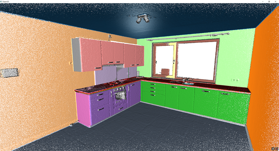
But is this the end? Noooo, never 😄! One last final step!

Clustering the remaining 3D points with DBSCAN

Finally, we go outside the loop, and we work on the remaining elements stored in rest that are not yet attributed to any segment. For this, a simple pass of Euclidean clustering (DBSCAN) should do the trick:

labels = np.array(rest.cluster_dbscan(eps=0.05, min_points=5))
max_label = labels.max()
print(f"point cloud has {max_label + 1} clusters")
colors = plt.get_cmap("tab10")(labels / (max_label if max_label > 0 else 1))
colors[labels < 0] = 0
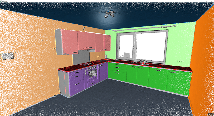
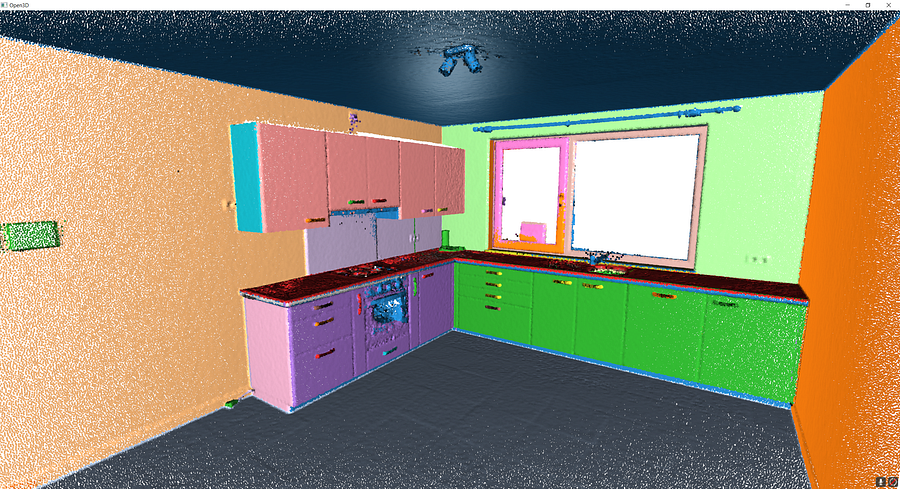
rest.colors = o3d.utility.Vector3dVector(colors[:, :3])

I employ the same methodology as before, no sorcery! I just make sure to use coherent parameters to have a refined clustering to get the beautiful rainbow kitchen you always dreamed of 🥳!

If you want to get it working directly, I also create a Google Colab script that you can access here: To the Python Google Colab script.

Conclusion

Massive congratulations 🎉! You just learned how to import and develop an automatic segmentation and visualisation program for 3D point clouds composed of millions of points, with different strategies! Sincerely, well done! But the path certainly does not end here, because you just unlocked a tremendous potential for intelligent processes that reason at a segment level!

Future posts will dive deeper into point cloud spatial analysis, file formats, data structures, object detection, segmentation, classification, visualization, animation and meshing. We will especially look into how to manage big point cloud data as defined in the article below.

The Future of 3D Point Clouds: a new perspective
Discrete spatial datasets known as point clouds often lay the groundwork for decision-making applications. But can they…towardsdatascience.com

Going Further

Other advanced segmentation methods for point cloud exist. It is actually a research field in which I am deeply involved, and you can already find some well-designed methodologies in the articles [1–6]. For the more advanced 3D deep learning architectures, some comprehensive tutorials are coming very soon!

1. Poux, F., & Billen, R. (2019). Voxel-based 3D point cloud semantic segmentation: unsupervised geometric and relationship featuring vs deep learning methods. ISPRS International Journal of Geo-Information. 8(5), 213; https://doi.org/10.3390/ijgi8050213 — Jack Dangermond Award (Link to press coverage)
2. Poux, F., Neuville, R., Nys, G.-A., & Billen, R. (2018). 3D Point Cloud Semantic Modelling: Integrated Framework for Indoor Spaces and Furniture. Remote Sensing, 10(9), 1412. https://doi.org/10.3390/rs10091412
3. Poux, F., Neuville, R., Van Wersch, L., Nys, G.-A., & Billen, R. (2017). 3D Point Clouds in Archaeology: Advances in Acquisition, Processing and Knowledge Integration Applied to Quasi-Planar Objects. Geosciences, 7(4), 96. https://doi.org/10.3390/GEOSCIENCES7040096
4. Poux, F., Mattes, C., Kobbelt, L., 2020. Unsupervised segmentation of indoor 3D point cloud: application to object-based classification, ISPRS — International Archives of the Photogrammetry, Remote Sensing and Spatial Information Sciences. pp. 111–118. https://doi:10.5194/isprs-archives-XLIV-4-W1-2020-111-2020
5. Poux, F., Ponciano, J.J., 2020. Self-learning ontology for instance segmentation of 3d indoor point cloud, ISPRS — International Archives of Photogrammetry, Remote Sensing and Spatial Information Sciences. pp. 309–316. https://doi:10.5194/isprs-archives-XLIII-B2-2020-309-2020
6. Bassier, M., Vergauwen, M., Poux, F., (2020). Point Cloud vs. Mesh Features for Building Interior Classification. Remote Sensing. 12, 2224. https://doi:10.3390/rs12142224

This article is derived from the originally published article in Towards Data Science.