


3D point cloud segmentation splits a raw scan into groups of points that belong together, so a floor, a wall or a single chair becomes an object you can query. Three classical families do the work: density clustering with DBSCAN, shape fitting with RANSAC, and region growing on surface normals. Open3D runs all three in Python.
A fresh scan looks fantastic, right up to the moment you try to do something with it and the whole thing goes quiet.
| What it is | Cutting a raw 3D scan into groups of points that belong together, so each part of the scene can carry a name |
| What you build | A two stage Open3D pass that fits and strips the dominant plane with RANSAC, then clusters the leftovers with DBSCAN and colors every cluster |
| Libraries | Open3D (segment_plane, cluster_dbscan, estimate_normals, KDTreeFlann) and NumPy |
| Worked on | Indoor scans read from a .ply file, with distance_threshold=0.02 for the plane and eps=0.05, min_points=10 for the clusters |
| Level | Beginner to intermediate. No training data and no GPU, a CPU handles the whole pass. |
Here is the path this guide takes, so you can jump straight to the part you need:
- What 3D Point Cloud Segmentation Really Means
- Segmentation Versus Semantic And Instance Labels
- The 3D Point Cloud Segmentation Method Families
- Density Clustering With DBSCAN
- Fitting Shapes With RANSAC
- Region Growing For Surfaces That Touch
- The Two Stage Pipeline In Python
- Tuning Parameters And Dodging The Common Pitfalls
- From Geometry To Names With Learned Segmentation
- Where 3D Point Cloud Segmentation Fits Next
- Frequently Asked Questions
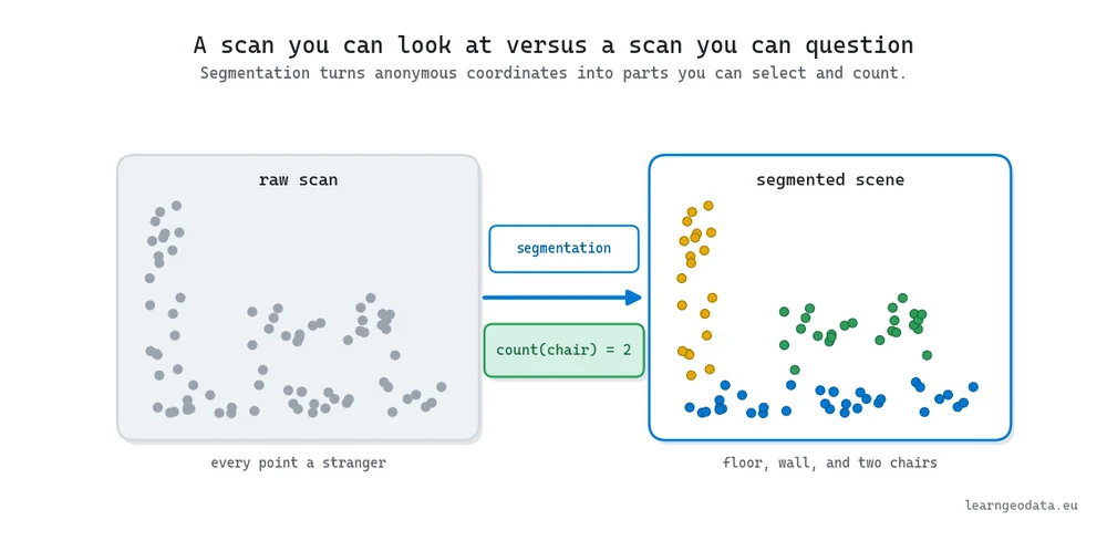
You want to click the floor and hide it, count the chairs, pull one machine off a factory scan for a report. Nothing happens, because to your software every point is a stranger to every other point.
That gap, between a scan you can admire and a scan you can interrogate, is exactly what 3D point cloud segmentation closes. This guide walks the whole toolbox in the order I would teach it, so you leave with the full map, not one clever trick.
What you’ll learn in this article:
- What segmentation is, and why it is the hinge of every 3D spatial AI workflow
- The difference between segmentation, semantic labels, and instance labels
- Which method family wins on your data, and the trade-off behind each choice
- Real Open3D code that fits a plane with RANSAC and clusters the rest with DBSCAN
- The parameters that decide your result, and the traps that quietly ruin it
Estimated reading time: 13 minutes
What 3D Point Cloud Segmentation Really Means
Let me put the problem in plain words. A raw cloud is a bag of coordinates, maybe with a color and an intensity value pinned to each point. There are no walls in that file, no floor, no chairs, only positions.
Segmentation draws lines through that bag so points that belong together land in the same group. Get it right and a group can carry a name. Get it wrong and you are back to eyeballing colors.
Why does this one move matter so much? Because everything downstream assumes it already happened. A quantity takeoff on a wall, a ground model with the trees stripped away, a digital twin of a single conveyor, each of them starts from parts, not from a pile.
🦚 Florent’s Note: For years my instinct was to compute every descriptor I could think of, thirty of them, and let the algorithm sort it out. That backfires fast. Distances stop meaning much once you stack that many dimensions, so four well-chosen signals routinely beat thirty lazy ones. Start with position plus surface normals, and add curvature or intensity only when a real confusion in your own data asks for it.
Segmentation Versus Semantic And Instance Labels
Segmentation, semantic segmentation and instance segmentation are three different jobs, and the one you need changes the tools you reach for. People say segmentation and mean any of them, which costs a lot of confused afternoons.
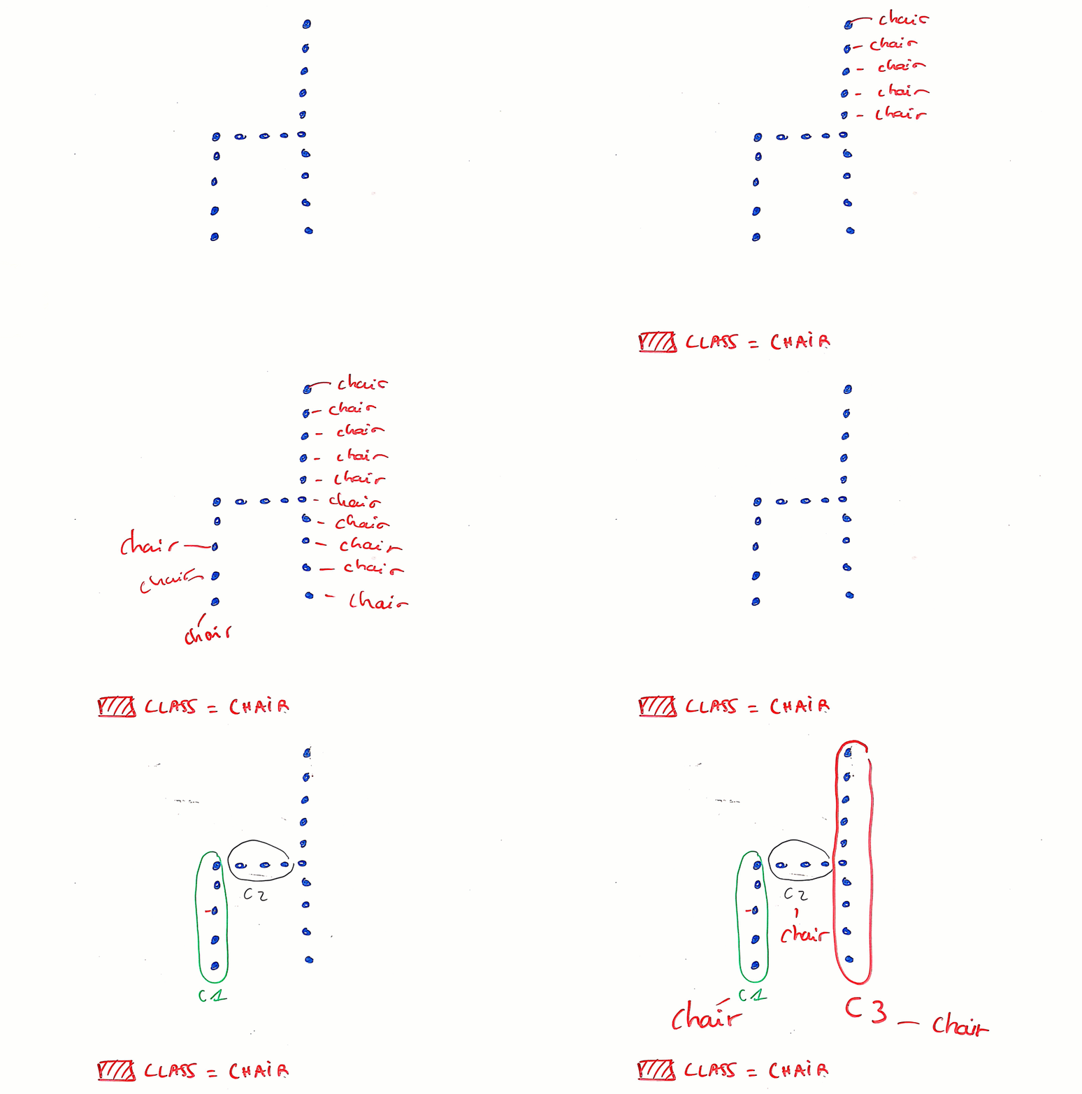
Plain segmentation groups points that belong together and stops there. You get cluster one, cluster two, cluster three, with no idea what any of them is, honest about geometry and silent about meaning.
Semantic segmentation adds a class name to every point. Now three separate chairs all carry the label chair, and the floor carries floor, so you can query the scene in words. Instance segmentation goes one step further and keeps the three chairs apart as chair one, chair two, and chair three, so you can count and address each object on its own.
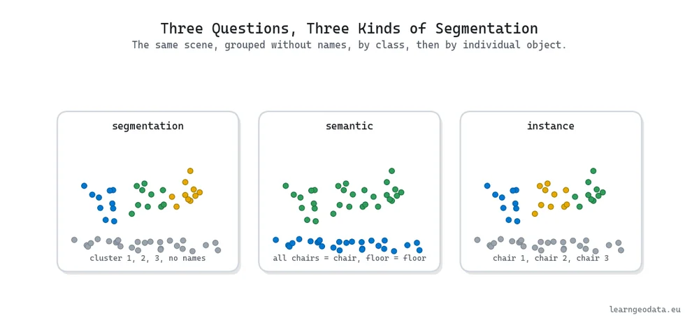
Which one should you aim for? It depends on the question. To remove the floor, plain grouping is plenty. To answer how many chairs, you need instance labels, and that is a harder, more expensive ask.
The 3D Point Cloud Segmentation Method Families
3D point cloud segmentation has no single best algorithm, only a small set of method families, each strong on a different kind of scene. Anyone who tells you otherwise is selling something.
Density clustering groups points that are packed tightly and calls the empty stretches noise. Shape fitting, led by RANSAC, hunts for a specific geometry like a plane or a cylinder. Region growing spreads outward from a seed while the surface stays smooth. Learned methods skip the hand-written rules and train a model to assign the labels for you.
So how do you choose? Let the question you can honestly answer about your data pick the tool for you.
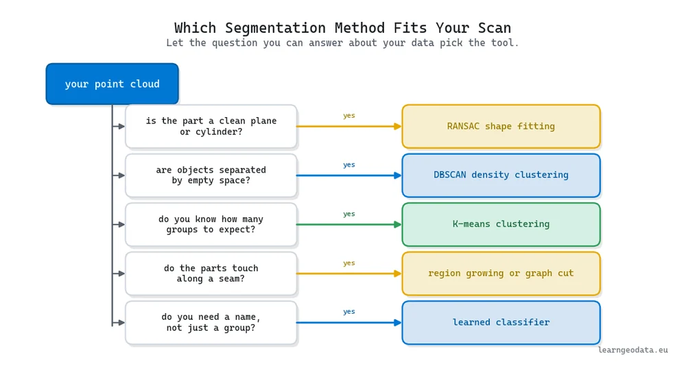
Notice that these families are partners, not rivals. A real pipeline chains a few of them, and the rest of this guide walks each one. For a broader tour of the methods, see our guide to 3D point cloud segmentation with Python.
🦥 Geeky Note: K-means is the clustering method plenty of people meet first, and it has one hard limit worth knowing early. It wants round, roughly equal blobs, so it hacks a long pipe run or a curb that wraps a corner into pieces that mean nothing physically. It also makes you guess K, the group count, up front, so setting K=6 on a room holding nine objects quietly fuses three of them. That is why so much point cloud work reaches past it for density-based clustering, which the scikit-learn clustering guide lays out beside a dozen alternatives.
Density Clustering With DBSCAN
DBSCAN is the density workhorse, and it fits scans beautifully because objects are dense while the air between them is empty. It never asks you for a group count. Instead it grows clusters wherever points crowd together and leaves the sparse gaps behind.
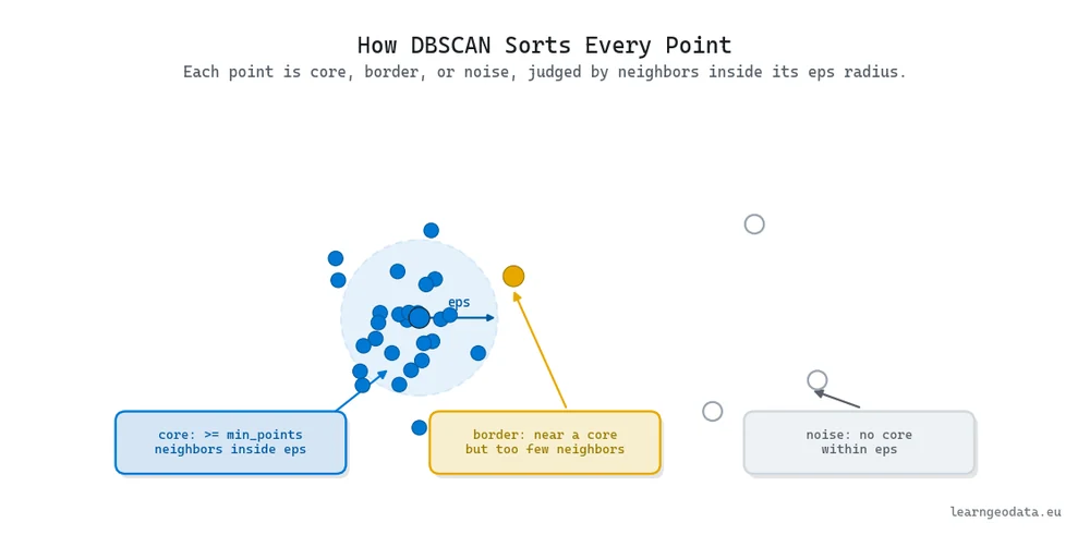
The idea rests on two numbers. The first is eps, the radius of the neighborhood around each point. The second is min_points, how many neighbors a point needs before it counts as sitting in a dense region.
With those two knobs, DBSCAN sorts every single point into one of three buckets. A core point has enough neighbors inside its radius. A border point sits near a core but lacks the neighbor count itself. A noise point has no core within reach at all.
That three-way sort is the whole algorithm, and it is why DBSCAN handles ragged, real-world shapes that K-means mangles. A long thin curb stays one object because its points form an unbroken dense chain, not because you told the method how many curbs to expect. For a hands-on walkthrough, see our Python guide to Euclidean clustering of 3D point clouds.
🌱 Growing Note: The descriptor space you run DBSCAN in decides what it can even separate. Cluster on raw position and a flat floor melts into a tilted loading ramp that touches it. Add a surface normal to each point, so the descriptor is now five numbers instead of three, and the two peel apart cleanly. You changed nothing about the algorithm, only what it was allowed to see.
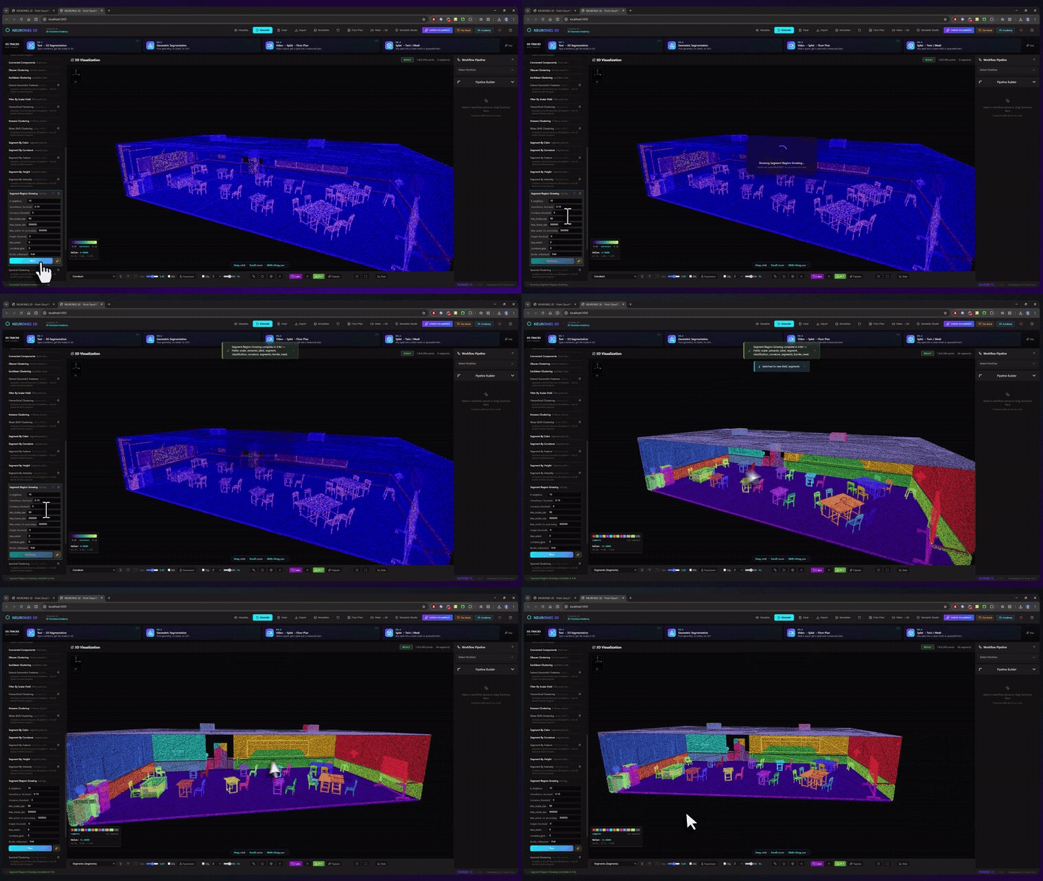
Fitting Shapes With RANSAC
RANSAC fits a shape you already have in mind, which is how you split parts that share an edge, like a floor and a wall meeting at a seam. Density grouping only works when a gap sits between your objects, and proximity thinking fails at a seam, because there the two really are close.
This is where you flip the question. Clustering asks which points are near each other. RANSAC asks which points fit a shape you already have in mind, and that change of framing is powerful.
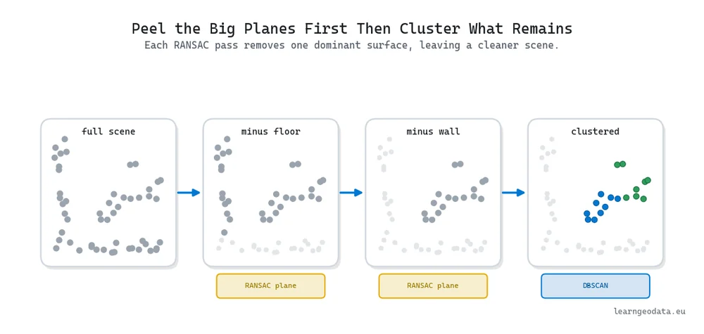
To pull a floor, RANSAC guesses a plane from three random points, counts how many of the rest fall within a threshold band, and remembers the score. Then it does that again, thousands of times, keeping whichever plane the largest crowd of points agreed with.
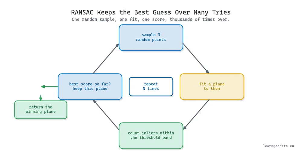
That majority-vote instinct came out of a 1981 paper by Fischler and Bolles, and it had nothing to do with rooms. They were locating a camera from noisy landmark matches and needed a method that could shrug off wrong answers. Four decades on, the same trick pulls a floor out of a cluttered scan. Our guide to 3D shape detection with RANSAC in Python fits planes and spheres step by step.
🪐 System Thinking Note: RANSAC and clustering compose into something bigger than either alone. Fit and strip the dominant planes first, then cluster only the messy remainder. You have turned one impossible problem over a million points into a short stack of small, clean ones, each a few thousand points you can actually inspect. That decomposition is the heart of every serious pipeline: never attack the mess whole, break it into parts you can each solve, then compose the answers back up.
Region Growing For Surfaces That Touch
Region growing is the third family, and it covers the blind spot DBSCAN and RANSAC share on gently curved surfaces that touch and flow into each other. The method spreads outward from a seed point for as long as the surface normals stay aligned.
You drop a seed point, then look at its neighbors one by one. A neighbor joins the region only when its surface normal points roughly the same way as the seed. The region spreads across a smooth surface and stops dead at any crease where the geometry turns.
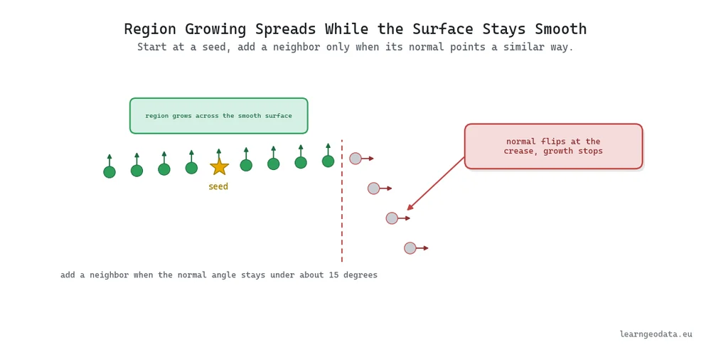
This is the method for a single continuous surface with a soft boundary, like a road that curves or a domed roof. It follows the shape of the thing rather than its density.
Here is region growing in practice, built on the surface normals you already estimated. You pick an unvisited seed, then let it recruit neighbors whose normal points nearly the same way, one hop at a time, until the smooth patch runs out and the walk stops on its own.
import open3d as o3d
import numpy as np

pcd = o3d.io.read_point_cloud("scan.ply")

# Region growing needs a normal at every point, so estimate them first.
pcd.estimate_normals(
    search_param=o3d.geometry.KDTreeSearchParamHybrid(radius=0.1, max_nn=30))
normals = np.asarray(pcd.normals)
tree = o3d.geometry.KDTreeFlann(pcd)

n = len(pcd.points)
labels = np.full(n, -1, dtype=int)     # -1 means not yet assigned
cos_thresh = np.cos(np.deg2rad(15.0))  # neighbors within 15 degrees may join
radius = 0.1                           # local neighborhood, in scan units
region = 0

for seed in range(n):
    if labels[seed] != -1:
        continue                       # already swallowed by an earlier region
    labels[seed] = region
    stack = [seed]
    while stack:                       # grow outward from the seed
        p = stack.pop()
        _, idx, _ = tree.search_radius_vector_3d(pcd.points[p], radius)
        for j in idx:
            # abs() because a normal and its flip describe the same surface.
            if labels[j] == -1 and abs(normals[p] @ normals[j]) >= cos_thresh:
                labels[j] = region
                stack.append(j)
    region += 1

print(f"Region growing found {region} smooth surface regions")
The cos_thresh is the real control here. Loosen it toward 30 degrees and a gently domed roof stays one region, tighten it toward 5 and the same roof splinters at every subtle ripple, so tune it to how smooth your surfaces actually are.
The Two Stage Pipeline In Python
The two stage pipeline in Python fits and removes the big planes with RANSAC, then clusters the leftovers with DBSCAN. That combination does real work indoors, where scenes are mostly planes and boxes.
Open3D ships both halves, so the whole pass is a short block rather than a project. It exposes plane fitting as segment_plane and density clustering as cluster_dbscan, both documented in the Open3D docs.
import open3d as o3d
import numpy as np

pcd = o3d.io.read_point_cloud("scan.ply")

# Stage 1: pull the dominant plane (floor, wall, or ceiling) with RANSAC.
plane_model, inliers = pcd.segment_plane(
    distance_threshold=0.02,   # a point within 2 cm of the plane is an inlier
    ransac_n=3,                # a plane is defined by 3 points
    num_iterations=1000,       # more guesses, steadier winner
)
print(f"Plane kept {len(inliers)} of {len(pcd.points)} points")

# Keep everything that is NOT on that plane.
remainder = pcd.select_by_index(inliers, invert=True)

# Stage 2: cluster the leftover points by density.
labels = np.array(remainder.cluster_dbscan(eps=0.05, min_points=10))
n_clusters = labels.max() + 1
print(f"DBSCAN found {n_clusters} clusters in the remainder")

# Color each cluster so you can see the split, noise stays black.
colors = np.zeros((len(labels), 3))
palette = np.random.default_rng(0).uniform(0, 1, (max(n_clusters, 1), 3))
for i, lab in enumerate(labels):
    if lab >= 0:
        colors[i] = palette[lab]
remainder.colors = o3d.utility.Vector3dVector(colors)
o3d.visualization.draw_geometries([remainder])
Two parameters steer the whole result. The distance_threshold sets how close a point must sit to count as part of the plane, and eps sets the radius DBSCAN grows clusters from. Scale both to your point spacing, tighter for a dense tripod capture, looser for a sparse mobile mapping pass.
One detail saves you a confusing bug. The cluster_dbscan call returns a label per point, and it marks noise with negative one, which is why the cluster count reads labels.max() + 1 rather than the number of distinct labels.
Run this on a tidy indoor scan and you get a colored, part-by-part model with zero training data, the honest place to start.
🦥 Geeky Note: The default num_iterations=1000 is generous for a single dominant plane, and you can often drop it to 200 or 300 with no visible loss on a clean scan. The math behind why so few random tries suffice is elegant: if roughly half your points sit on the target plane, the odds of never sampling three inliers across a thousand tries are astronomically small. Raise the count only when the target surface is a thin minority of the cloud.
Tuning Parameters And Dodging The Common Pitfalls
Parameter tuning is the part tutorials skip, and it decides whether your pipeline survives scan number two. You can read any of these algorithms in an afternoon. Building the instinct for what each parameter does to your scans takes months of hands-on repetition.
Take eps in DBSCAN. It is a single number, and it has three completely different personalities depending on how you set it against your point spacing.
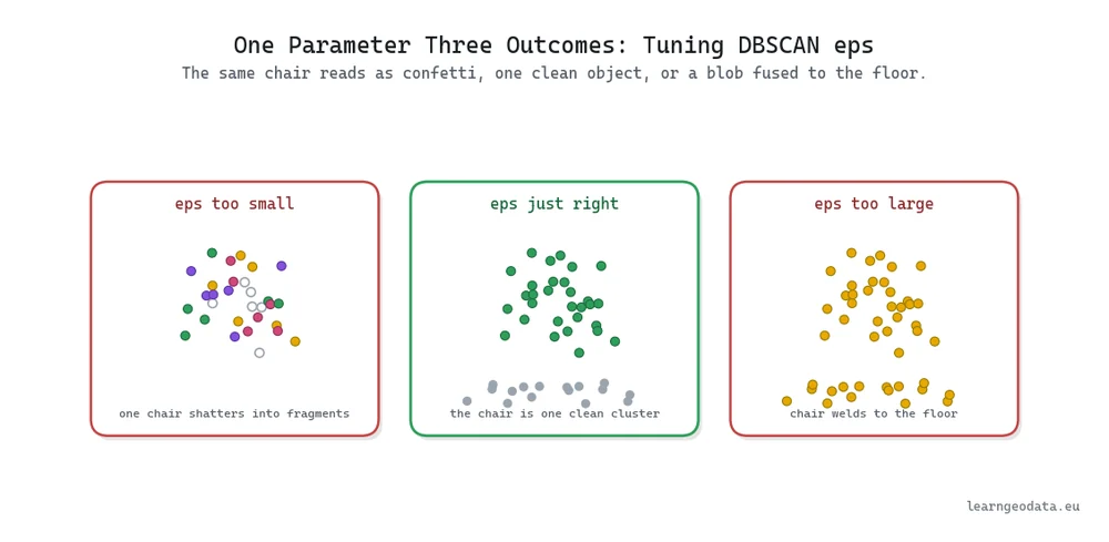
The trap that catches people is hard-coding a value. You tune eps=0.05 on a scan captured at one centimeter spacing, it works, you ship it, and then you feed the same pipeline a mobile-mapping scan at five centimeter spacing. DBSCAN now labels almost everything as noise and hands back an empty result that looks exactly like a bug.
So scale your parameters to point spacing, never to a memorized constant. A quick habit that pays off is to estimate the median nearest-neighbor distance of a new cloud and set eps to a small multiple of it, so the pipeline adapts instead of breaking.
The same discipline applies to the RANSAC distance_threshold: too tight splits a slightly noisy wall into several thin planes, too loose grabs the floor plus half the objects on it as one greedy surface.
From Geometry To Names With Learned Segmentation
Everything so far groups points and structures them, but none of it knows what a wall actually is. Geometry can tell you a cluster is dense and connected, not that it is a chair. Attaching a name is the last jump, and it is the one machine learning owns.
The honest way to learn it is not to reach for a heavy neural network on day one. Start with a descriptor-plus-classifier approach: compute a handful of informative signals for each point, feed them to a trained classifier, and let it decide the class one point at a time.
Which signals? Height above the ground, the local surface normal, and local roughness carry more meaning than raw position ever could. A tabletop and the floor are both flat and horizontal, so the bare coordinate tells a classifier nothing, while those three descriptors encode the context that pulls them apart.
🌱 Growing Note: When hand-built descriptors run out of road on varied, cluttered scenes, learned representations take over, and the graph view of a cloud becomes the bridge. Architectures collapse millions of raw points into a few thousand superpoints first, then reason over those instead. The Superpoint Transformer is a clear example of that lineage, and it is where the density and graph ideas from this guide reappear at scale.
Run the classifier across every point and you get a labeled scene rather than a labeled dot, the top of the ladder: parts that mean something in plain words. For a full learned pass, see our tutorial on 3D semantic segmentation with the Superpoint Transformer.
Where 3D Point Cloud Segmentation Fits Next
Segmentation is one stop on a longer road that runs from capturing reality to reasoning over it. Each stage leans on the one before it, so it helps to see the whole route.
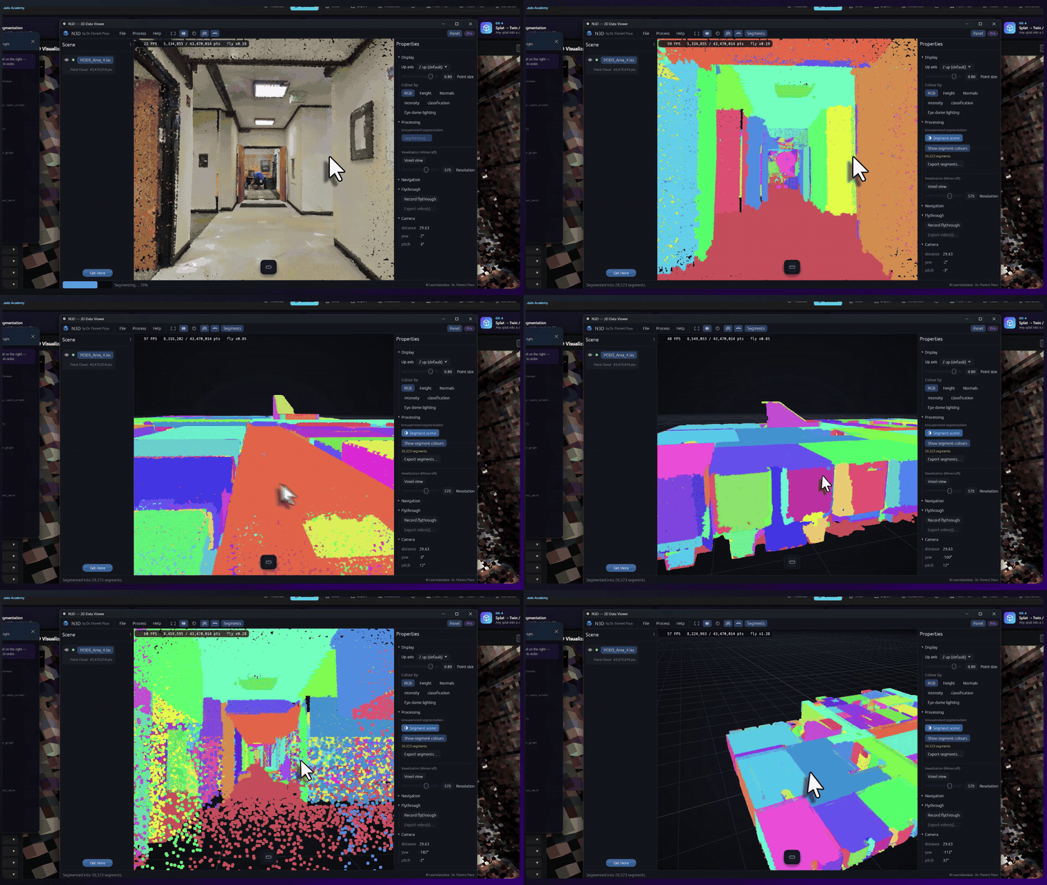
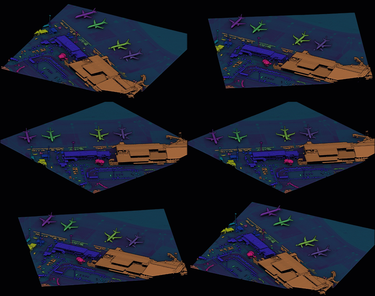
Upstream sits capture and cleaning, covered in LiDAR and point cloud processing, where the raw data that lands on your desk gets ingested and prepared. The full map from sensing to reasoning lives in the 3D Spatial AI with Python guide.
Downstream, 3D deep learning picks up where hand-built descriptors run out and teaches networks to learn the representation themselves. From there, semantic and spatial AI with scene graphs closes the loop with open-vocabulary labels a machine can reason across.
🦚 Florent’s Note: Here is the part that matters in the age of AI, and I mean it plainly. A segmentation app hands you a button that says segment, and it works right up until it does not, and then you are stuck. The person who knows the RANSAC threshold, the DBSCAN radius, and the descriptor that splits a tabletop from a floor is the one who builds the button and decides what it does. That knowledge is worth more now, not less, because the tools amplify whoever understands them and quietly sideline whoever only clicks.
If you want to build that depth in a structured way, with production code and the parameter intuition you cannot get from one article, that is exactly what the 3D AI Program is built to teach. It treats segmentation not as a script you rerun by hand but as an engine you understand and own.
The fastest way to make this click is to build one small version yourself, on the scan already on your drive: wire the two-stage pass into a single loop, color each part, and see the split. The gentlest guided entry, with a real scan and starter code, is the 3D Spatial AI free mission.
So which scan is on your drive right now, the clean structured one that RANSAC and DBSCAN will crack in an hour, or the messy varied one that pulls you into learned labels, and are you ready to be the person who understands what runs underneath the button?
Frequently Asked Questions
How Do I Start Segmenting A 3D Point Cloud In Python?
Begin with Open3D, because it ships plane-fitting RANSAC as segment_plane and density clustering as cluster_dbscan out of the box, and it pairs cleanly with NumPy. Load your cloud, pull the dominant plane, remove it, then cluster the remainder. For a guided first run with a real scan and starter code, the 3D Spatial AI free mission walks you through the whole loop.
What Is The Difference Between Segmentation And Semantic Segmentation?
Plain segmentation groups points that belong together and gives you anonymous clusters, so you get cluster three, not chair. Semantic segmentation assigns a learned class name to every point, so the output is a scene you can query in words, and instance segmentation goes further by keeping each object separately addressable. Building that naming depth end to end is the focus of the 3D AI Program.
Should I Use DBSCAN Or RANSAC For My Scan?
Use RANSAC when you are after a clean geometric shape like a plane or cylinder that clustering would break apart, and use DBSCAN when your objects are separated by empty space. The strongest indoor pipeline uses both in sequence: RANSAC strips the big planes first, then DBSCAN clusters what remains. The majority-vote idea that makes RANSAC resist outliers comes from the Fischler and Bolles paper.
How Do I Choose DBSCAN eps And min_points?
Scale them to your point spacing rather than copying a constant, because a value tuned at one centimeter resolution will label a five centimeter scan as pure noise. For a room near one centimeter spacing, eps around 0.05 meters and min_points near 10 is a sensible first guess before you tune. The scikit-learn clustering guide shows how the parameters change the behavior across methods.
Do I Need Deep Learning For 3D Point Cloud Segmentation?
Not to start, and often not at all for clean, structured scenes, where RANSAC plus DBSCAN gets real work done with zero training data. Reach for learned methods when scenes get varied and cluttered and a name matters more than a group. Transformer approaches like the Superpoint Transformer show where the field is heading once hand-built descriptors run out of road.

