

3D deep learning trains neural networks on unordered point sets rather than pixel grids. Because a scan has no fixed row and no fixed neighbor, the network runs the same small function on every point, then folds the results with a symmetric pool so input order stops mattering. PointNet, PointNet++ and KPConv each answer that one constraint differently.
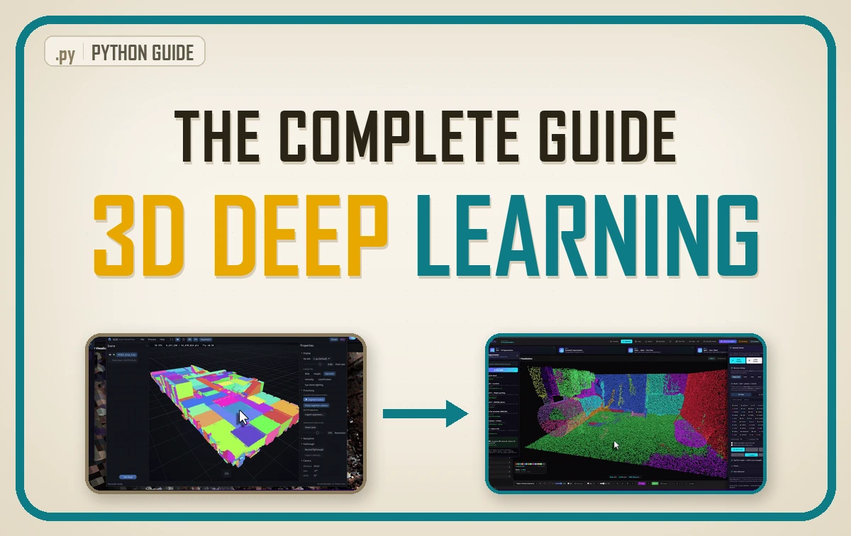
| What it is | Neural networks that learn on unordered 3D point sets instead of pixel grids |
| What you build | A tiny PyTorch point network, a shared per-point function plus a symmetric max pool, and the shuffle test that proves the output does not move when the input order does |
| Libraries | PyTorch (torch, torch.nn), and scikit-learn for a classical random-forest baseline |
| Worked on | Fixed-size samples of 1024 or 4096 points, cut from room scans that run from two million points down to 300,000 |
| Level | Intermediate. A CPU is enough for the tiny model and the shuffle test. |
So what actually breaks when you hand a scanner’s loose bag of coordinates to a network built for tidy pixel grids?
The route starts with what breaks, moves to the single operation that fixes it, and ends with the three architectures built on top:
- Why Point Clouds Break Ordinary Neural Networks
- What Permutation Invariance Actually Means
- The Tiny PyTorch Model That Proves It
- The One Training Step That Teaches Per-Point Labels
- Why Data Preparation Decides Your 3D Deep Learning Model
- PointNet PointNet++ And KPConv Compared
- What A Trained Model Hands You
- The Order To Learn 3D Deep Learning In
- Where 3D Deep Learning Fits In Your Spatial AI Path
- Start Training Your First Point Cloud Model This Week
- Frequently Asked Questions
You can point a pretrained image classifier at a folder of photos and have working predictions before your coffee cools. Try the same trick on a laser scan of a stairwell, and every instinct you trusted quietly stops working.

Why 3D Deep Learning Feels Different
That gap is where 3D deep learning starts, and it catches almost everyone who crosses into three dimensions. A network built to read a grid of pixels cannot read a loose bag of coordinates. Once you understand why, the rest of the field snaps into an order you can actually follow.
So this guide is the whole map, start to finish. What breaks, what fixes it, how to prepare your data without lying to yourself, the three architectures worth your time, and the order to learn them in.
What you will learn in this article
- Why an unordered set of points jams an ordinary neural network, and the single operation that unjams it
- How to write a permutation-invariant max-pool in a dozen lines of PyTorch and prove it holds
- The data preparation step that quietly decides whether your model learns or memorizes noise
- How PointNet, PointNet++, and KPConv answer the same question three different ways
- A concrete order to learn all of it in, from a first tensor to your own architecture
Why Point Clouds Break Ordinary Neural Networks
Start with a photo, since that is the comfortable case. A photo is a grid, and row twelve column forty is always the same pixel with the same neighbors. A convolution can march across it precisely because every pixel sits in a fixed, knowable neighborhood.
Now swap in a room captured by a scanner. What comes back is a list of XYZ triplets, maybe two million of them, in whatever sequence the hardware happened to fire. There is no row twelve. There is no fixed neighbor.
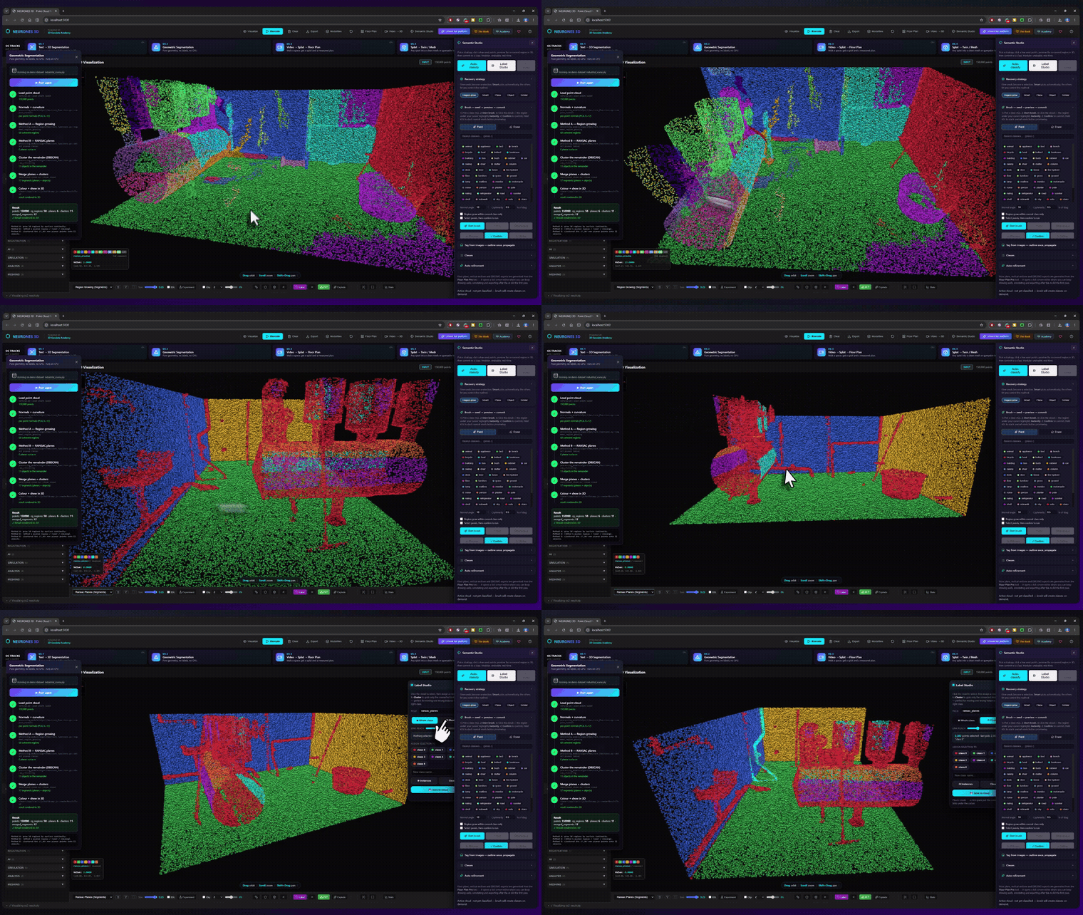
Here is the part that surprises people. Shuffle every line of that file and you are looking at the exact same room, unchanged in every physical way. The geometry did not move a millimeter.
So what happens when you push that list into a plain fully connected network? It reads position number five as one specific input slot with its own weights. Reorder the file, and every slot now holds a different point, so the network computes something new for a room that never moved. A chair has to register as a chair whether its points arrive front to back or scrambled, and a slot-based network cannot promise that.
What Permutation Invariance Actually Means
The fix is cleaner than the problem, which is my favorite kind of fix. The property you want has a name, permutation invariance, and it means the output must not depend on input order.
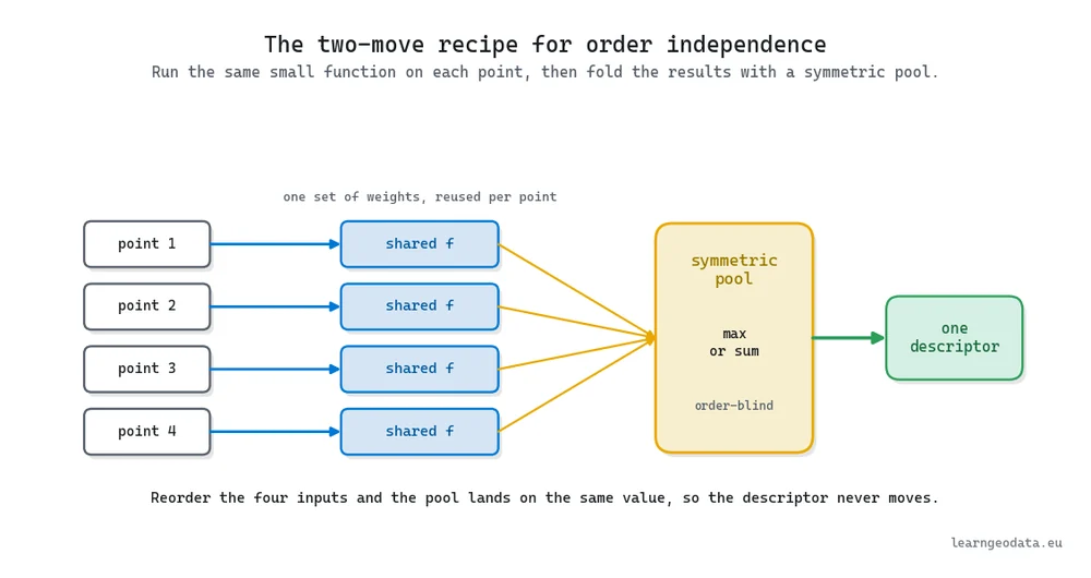
You buy it with a two-move recipe. First, run the same small function over each point on its own, so no single point gets a privileged slot. Second, fold those per-point results together with a symmetric operation that returns the same value no matter how you list its inputs.
Which operations are symmetric, and which quietly are not? A max lands on the same value whichever order you read it in. So does a sum, and so does a mean. Concatenation does the opposite: it cares deeply about which value sits in which slot, so it shatters the invariance you just built.
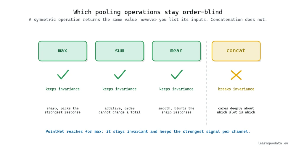
PointNet reaches for the max, and there is a reason. A mean keeps the invariance but blunts the sharp responses, and a max keeps the strongest signal per channel while staying order-blind. That single decision let PointNet train on raw points, and it still holds up nearly everything built since.
🦥 Geeky Note: The pooling here is a channel-wise max across all N points, each lifted to a 1024-dimensional vector by the shared perceptron. Drop the descriptor width from 1024 to 256 and you trade richness for speed, and the invariance survives untouched. The max is the load-bearing line, not the width you pick around it.
The Tiny PyTorch Model That Proves It
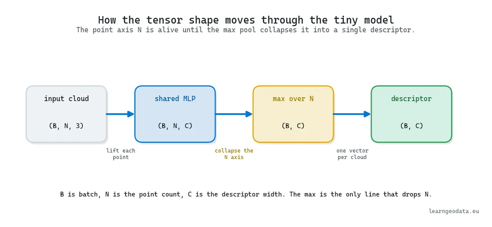
Let me show this small enough to read in one breath. The module below lifts every point through a shared multilayer perceptron, meaning the same weights process each point separately, then squashes the entire set into a single descriptor with a max across the point axis.
The last few lines are the honest part. They shuffle the input and check the output did not budge.
import torch
import torch.nn as nn


class MaxPoolPointNet(nn.Module):
    """Turn an unordered set of points into one order-independent descriptor."""

    def __init__(self, in_dim=3, width=64, code=1024):
        super().__init__()
        self.per_point = nn.Sequential(
            nn.Linear(in_dim, width),
            nn.ReLU(),
            nn.Linear(width, code),
        )

    def forward(self, cloud):                  # cloud: (B, N, in_dim)
        lifted = self.per_point(cloud)         # (B, N, code), same weights per point
        descriptor, _ = lifted.max(dim=1)      # (B, code), max across the N points
        return descriptor


net = MaxPoolPointNet()
points = torch.rand(1, 512, 3)
reordered = points[:, torch.randperm(512), :]
assert torch.allclose(net(points), net(reordered), atol=1e-6)   # order changes nothing
The line that earns its keep is descriptor, _ = lifted.max(dim=1). Everything above it is an ordinary PyTorch network you could have written for tabular data. That one max over the point axis is the entire reason the descriptor comes out identical after a shuffle.
It helps to watch the tensor shape as it travels, because the point axis is where the magic hides. The cloud goes in as (B, N, 3), the shared perceptron lifts it to (B, N, C) while keeping every point separate, and only the max collapses that middle axis into a single (B, C) descriptor per cloud.
If the assert passes on your machine, you have just proven permutation invariance by hand. That is worth more than reading ten explanations of it, and it takes about thirty seconds to run.
The One Training Step That Teaches Per-Point Labels
The shuffle test proved the descriptor holds still. It did not make the network right about anything, since a fresh model just emits noise. Training is the part that pushes its guesses toward the truth, and the smallest honest version of it is a single step: predict, measure the miss, nudge the weights.

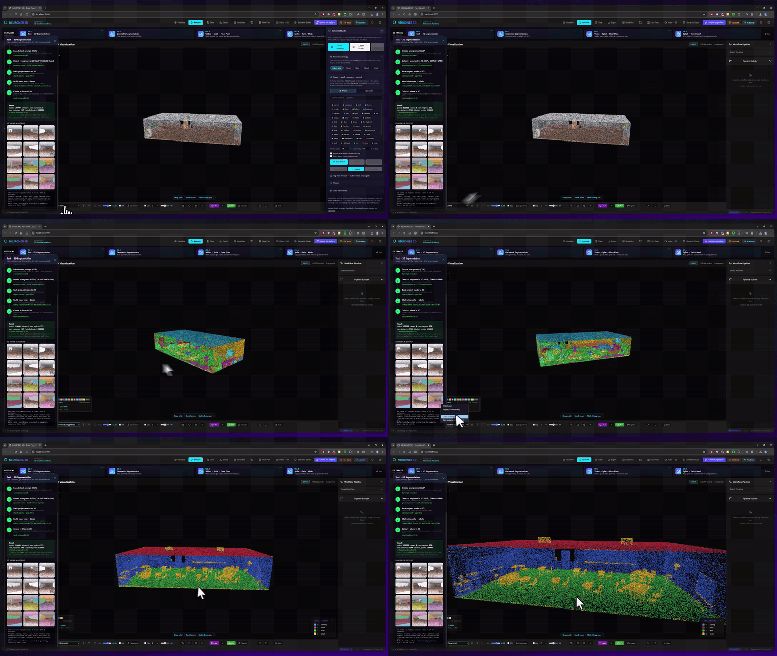
Trade the one global descriptor for a per-point head, and the same shared perceptron now emits a class score row for every point instead of one vector for the whole cloud. That is exactly the segmentation output you are after, a label sitting on each point.
import torch
import torch.nn as nn


class PerPointHead(nn.Module):
    """The shared-MLP idea again, but score every point instead of pooling to one vector."""

    def __init__(self, in_dim=3, width=64, num_classes=5):
        super().__init__()
        self.per_point = nn.Sequential(
            nn.Linear(in_dim, width),
            nn.ReLU(),
            nn.Linear(width, num_classes),
        )

    def forward(self, cloud):              # cloud: (B, N, in_dim)
        return self.per_point(cloud)       # (B, N, num_classes), one score row per point


model = PerPointHead(num_classes=5)
optimizer = torch.optim.Adam(model.parameters(), lr=1e-3)
loss_fn = nn.CrossEntropyLoss()

cloud = torch.rand(4, 1024, 3)             # (B, N, 3), a batch of prepared samples
labels = torch.randint(0, 5, (4, 1024))    # (B, N), the true class of each point

logits = model(cloud)                                        # (B, N, 5)
loss = loss_fn(logits.reshape(-1, 5), labels.reshape(-1))    # flatten points, then score
optimizer.zero_grad()
loss.backward()                            # gradients: how each weight moved the loss
optimizer.step()                           # walk every weight a small step downhill
The pair carrying the whole lesson is loss.backward() and optimizer.step(). The loss measures how far the per-point guesses sit from the labels, and that pair walks every weight a small distance down the gradient. Loop it over batches and the guesses drift toward the truth.
Notice the reshape too. Cross-entropy wants a flat list of point scores against a flat list of labels, so you fold the batch and point axes together, judge every point at once, and let one number cover the whole cloud. Get that loop running on toy tensors first, because the real work is feeding it clouds that were prepared honestly. Producing those per-point labels in the first place is its own task, and our guide to 3D point cloud labeling in Python covers it.
Why Data Preparation Decides Your 3D Deep Learning Model
Data preparation decides your 3D deep learning model because the hours you pour into cleaning and shaping clouds will outweigh the hours you spend fitting anything, and when the shaping is wrong, no architecture rescues you. That is the truth the polished tutorials skip past.
Think about what a network like PointNet demands at the door. Every sample the same size, often 1024 or 4096 points, recentered and normalized, sometimes with color or normal channels riding alongside the raw XYZ. Your scans offer none of that. One room hands you two million points, and the next has barely 300,000.
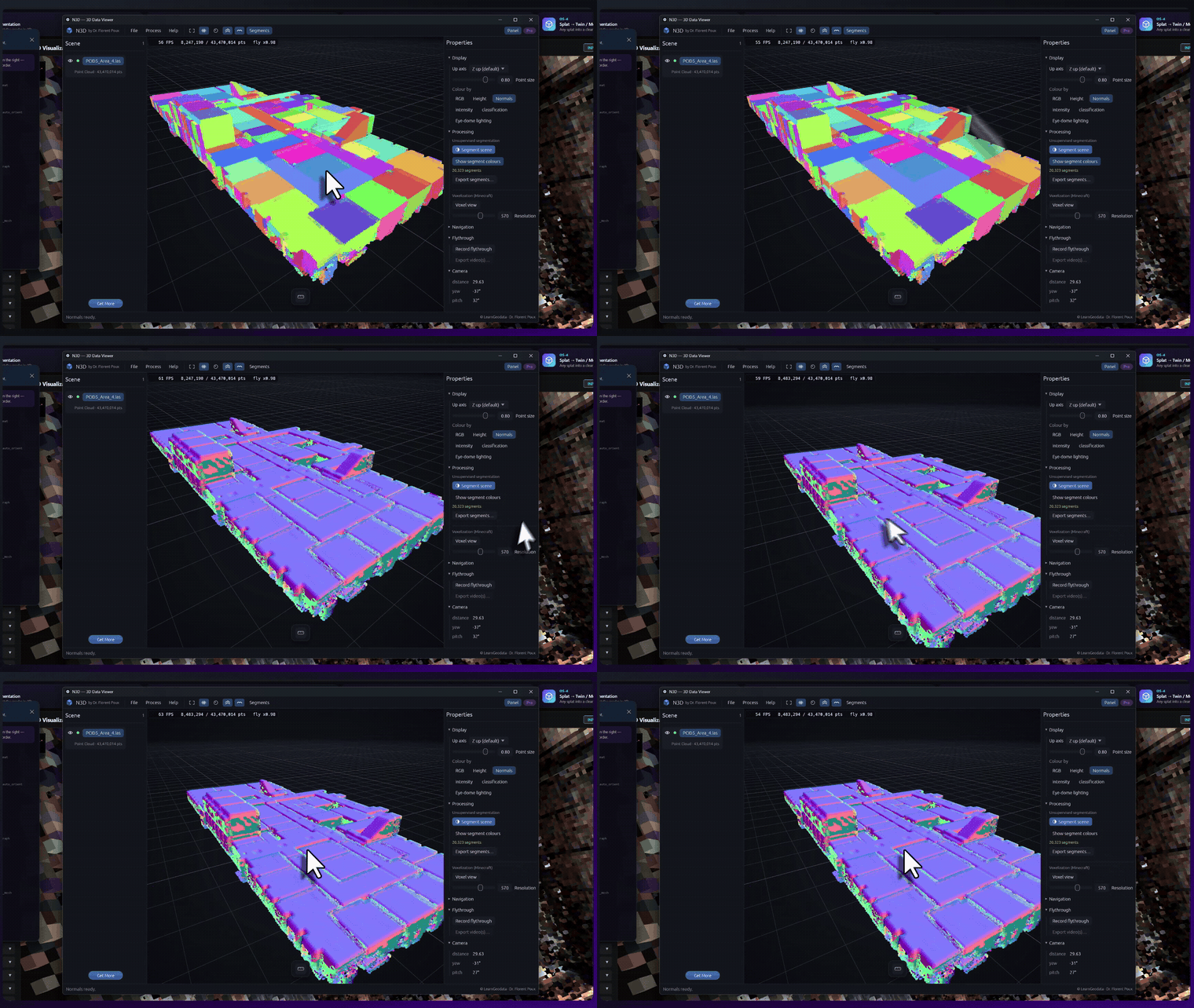
So preparation is not a chore you rush through. It is the part that quietly decides your ceiling. Two steps deserve special care, and beginners underestimate both. Our guide to point cloud data preparation for 3D deep learning walks the full prep pipeline.
Sampling A Scan Down To A Fixed Size
You cannot feed a variable point count into a fixed model, so you sample down to a set size. The lazy way is random downsampling, and it works until it does not. Random keeps clumps where the cloud was dense and leaves gaps where it was thin, so a corner of your object can vanish.
Farthest point sampling fixes that. It picks each new point to be as far as possible from the ones already chosen, so the survivors spread evenly across the shape instead of piling up.
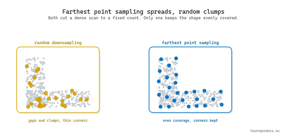
Is farthest point sampling slower? Yes, noticeably, because each pick scans the remaining points. For a 1024-point sample the cost is nothing you will feel, and the even coverage pays you back at training time.
Normalizing Coordinates So Training Moves
Now the step that once cost me a full week. A network fed raw coordinates in meters, running from roughly minus fifty to plus sixty, will often refuse to train at all, with the loss sitting flat as a table.
The fix is two operations. Center every cloud on its own centroid so it sits at the origin, then scale it so it fits inside a unit sphere. Suddenly every axis lives in a tidy range near zero, and the same architecture that sat dead now converges.
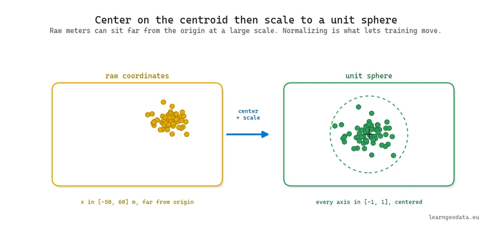
During training you also augment: random rotations about the vertical axis and a little jitter, so the model learns the shape rather than one frozen pose. Get any link in that chain wrong and the failure is sneaky, since the loss drops, training accuracy looks respectable, and the thing generalizes to nothing.
🦚 Florent’s Note: That input-scale bug is the dullest on the whole list, and it taught me more than any of them. I lost a week to a network that would not budge for a hundred epochs, and the cause was coordinates in meters that never got normalized. Now the first line of every prep script centers on the centroid and rescales into a unit sphere, no exceptions, because the same model on raw meters teaches you nothing but frustration.
🌱 Growing Note: Do not start on point clouds. Build a plain classifier on six or seven handcrafted descriptors first, normals plus curvature plus height above ground, and train it in scikit-learn on a labeled scan. You get a real baseline in an afternoon, and every deep model afterward has a number to beat. A network that cannot clear a random forest on the same data is telling you the prep is broken, not the architecture.
PointNet PointNet++ And KPConv Compared
All three ask one question: how do you learn descriptors on an unordered set of points? They answer in three flavors, and the lineage tells you which to reach for and, more usefully, which to learn first.
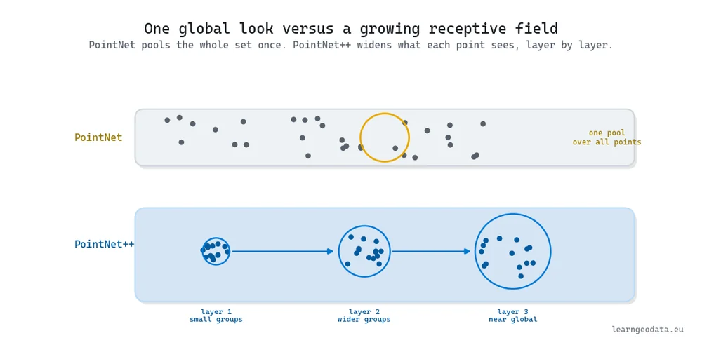
PointNet, published by Qi and coauthors in 2017, is the clean place to begin. Every point runs through the shared perceptron you already met, then a single global max pool folds the whole set into one vector describing the object. Read the original PointNet paper once you have done the data prep by hand, since it names every piece you just wrestled with.
Its weakness sits right in the design. That lone global pool sees the whole and misses the parts, so fine local structure slips past it.

So the same authors patched their own model. PointNet++ runs PointNet inside a hierarchy, applying it to small local groups, pooling those, then repeating on the pooled result. It builds descriptors from local up to global, the way a convolutional network stacks edges into objects.
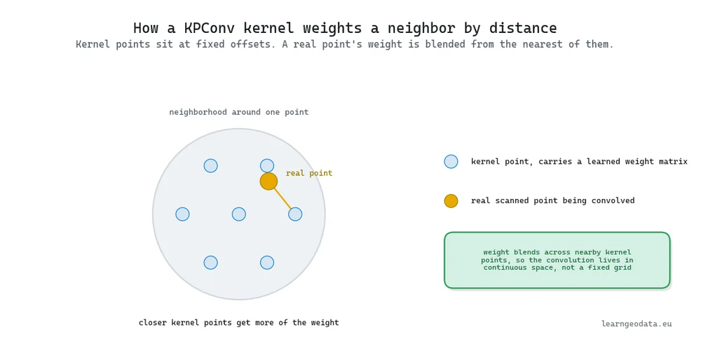
Then KPConv swung differently. Instead of pooling neighborhoods, it defines a genuine convolution for points, using kernel points placed at fixed offsets that weight nearby points by distance. A real scanned point gets its contribution blended across the closest kernel points, so the convolution lives in continuous space rather than on a fixed grid.
I nearly told you to start with PointNet++, since it is the stronger model you will reach for in practice. Then I caught myself, because that is backward. Learn the simple invariant first, and the hierarchy reads as an obvious next move rather than a black box. For a build-along, our step-by-step guide to a 3D object recognition algorithm puts one of these networks to work.
🪐 System Thinking Note: Notice what you really learned in the max-pool section. Apply a shared function per element, then combine with a symmetric operation, and you get a network that respects an unordered set. That pattern is not stuck to point clouds, since the same shape drives networks over molecules, graphs, and any collection where order carries no meaning. Learn it once as geometry and you own a tool that transfers far past the scan on your screen.
🦥 Geeky Note: KPConv’s kernel is a little cloud of roughly fifteen positions arranged inside a sphere, each carrying its own learned weight matrix. That is the trick that lets a convolution sit in continuous 3D space, and it is why KPConv stays steady when point density swings across an aerial or mobile scan.
What A Trained Model Hands You
Let us ground this, since the point of the whole stack was never the papers. You prep a scan into fixed-size normalized samples, run it through a trained PointNet or KPConv, and receive a class on every point: ground, building, vegetation, vehicle.
Those per-point classes are the raw material behind a city digital twin, a hands-off progress check on a building site, or a vehicle’s read of the road ahead. Label one room reliably and the same recipe scales to a district, then a country.
But the output is only as trustworthy as the signal going in. Bare coordinates on a rooftop and bare coordinates on a paved street can read almost identically to a network, since both are just flat patches. Fuse the scan with aligned imagery so each point also carries color, and you hand the model something real to separate on.
The Order To Learn 3D Deep Learning In
The fastest way to stall in 3D deep learning is to open a KPConv repository on day one and drown. So where does a beginner actually start? Not at the top.
Here is the order that works, easy rung first. Build a classical baseline so you have a number to beat. Build a plain training loop so the 3D models stop feeling like magic. Code PointNet yourself, since it teaches the one invariant everything reuses. Then, and only then, reach for the density-aware architectures, and reach for them as a library call rather than a from-scratch rebuild.
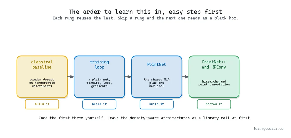
Why borrow the last rung instead of building it? Because the difficulty jump from PointNet to KPConv is steep, and nobody hands you a medal for starting at the hard end. For the wider set of resources and roadmaps, see our 3D deep learning essentials guide.
🌱 Growing Note: You do not have to rebuild these to run them. Open3D-ML bundles working PointNet++ and KPConv alongside loaders for common benchmarks, so you train on real data and read the reference code together. Code PointNet yourself to learn the internals, and treat KPConv as an import at first, since the honest goal is understanding the field, not proving you can suffer.
🦚 Florent’s Note: My rule when a shiny new architecture drops: do not rebuild the pipeline around it. Freeze your data prep and your evaluation harness, swap only the model, and measure the honest delta. Nine times in ten the real gain is a fraction of the abstract promise, and now you can prove it instead of feeling it. That one habit separates a practitioner who compounds from one the field keeps knocking flat.
Where 3D Deep Learning Fits In Your Spatial AI Path
3D deep learning sits in the middle of a spatial AI path, one stop on a longer route. The full map lives in the 3D Spatial AI with Python complete guide, which lays out the road from raw sensing through to reasoning about whole scenes.
Two natural clicks sit on either side of this one. Before you train anything, you want clean structured point groups, which is the job of 3D point cloud segmentation and clustering in Python, where plane fitting and density clustering carve a raw scan into parts a network can later learn to reproduce and outdo. After you can label points, the frontier is meaning, and semantic and spatial AI with scene graphs in Python takes over once single-point classes run out.
When you want the training loop, the debugging instincts, and the thousand small choices a paper never spells out, structured teaching earns its keep. The 3D Spatial AI Program is where I teach this end to end, from raw cloud to trained model, with the parameter intuition you cannot get from a single article.
Start Training Your First Point Cloud Model This Week
Reading about invariance is not what makes it stick. Running it once is.
So run the small loop this week. Prep a real scan into fixed-size normalized samples, fit a bare PointNet on a tidy benchmark, and label every point. Leave PointNet++ and KPConv alone until that first loop runs end to end on your own machine, because the simpler model teaches the mechanics the fancier ones reuse.
If you want a first real 3D Python task to run right now, the free mission hands you one to build this week. And when you are ready to go deep, the 3D Spatial AI Program takes you from this first loop all the way to designing your own architectures.
So which will you reach for first: the classical baseline that gives you a number to beat, or the network that learns the descriptors you used to design by hand?

Frequently Asked Questions
Why Can’t A Standard Neural Network Read A Point Cloud?
An ordinary network treats each input position as a fixed slot with its own weights, and a point cloud has no fixed order, so reshuffling the same points produces a different answer for the same geometry. The fix is permutation invariance through a symmetric pooling operation, introduced in the PointNet paper and kept by nearly every point model since.
Which 3D Deep Learning Model Should You Learn First?
Start with PointNet, always. It carries the single idea, order-independent pooling, that the later models build on, so learning it turns PointNet++ and KPConv into small steps rather than fresh mountains. If you want that groundwork taught in order, the 3D Spatial AI Program walks it from a first tensor to your own architecture.
How Important Is Data Preparation For Training PointNet?
It matters more than the architecture you pick. Sampling to a fixed point count, centering, scaling to a unit sphere, and augmenting with rotation and jitter decide whether the model learns the shape or memorizes noise. Practice it against real benchmark loaders in Open3D-ML rather than a toy set that hides the hard parts.
Does 3D Deep Learning Work On City-Scale Outdoor LiDAR?
Yes, and the density-aware models were built for exactly that. KPConv handles the uneven point density of aerial and mobile LiDAR well, because its kernel points weight neighbors by real distance rather than assuming a fixed grid, which is why it copes with scans that thin out with range.
Do You Need A GPU To Learn 3D Deep Learning?
To learn the concepts, no. You can prototype the tiny max-pool model and a small training run on a CPU, and the shuffle test in this guide runs in seconds without one. For full-resolution benchmarks and hierarchical models you will want a GPU, and you can start that step with a free run on the free mission.

