

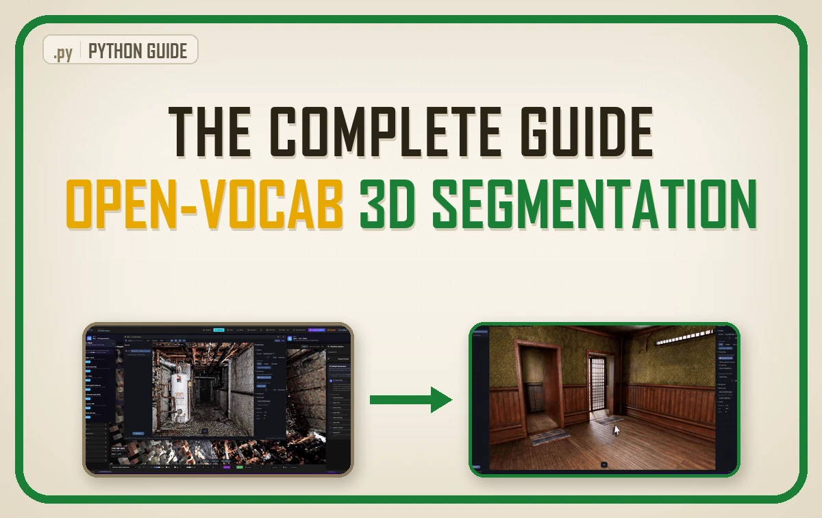
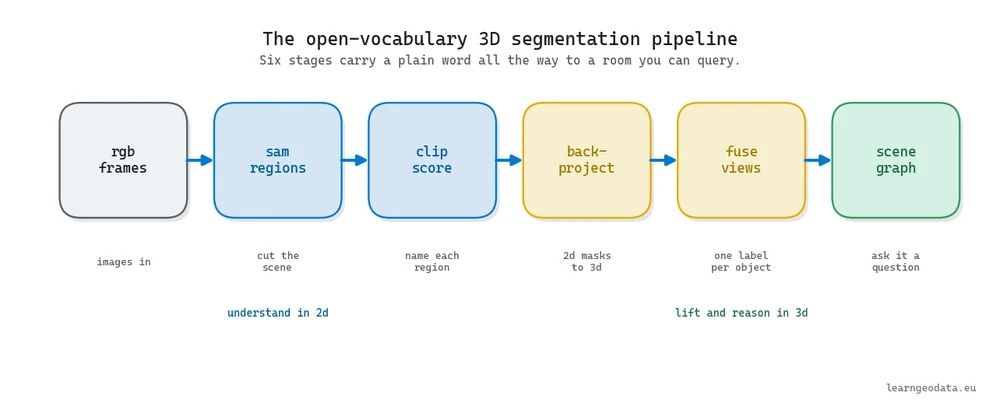
Open-vocabulary 3D segmentation labels a point cloud with any word you type, without training a 3D network. Segment Anything cuts rendered views into regions, CLIP scores each region against your text, and the winning label projects back onto the points. Fusing several views settles the disagreements, and the labeled objects assemble into a queryable scene graph.
| What it is | Labeling a point cloud with any word you type, with no 3D network trained |
| What you build | A pipeline that cuts rendered views into regions, scores each region against your word, lifts the winner back onto the points, and assembles the named objects into a queryable scene graph |
| Libraries | Segment Anything (vit_h), open_clip ViT-B-32 on laion2b_s34b_b79k, DINOv2, NetworkX, Open3D, NumPy |
| Worked on | A full indoor building capture, dense enough that one scan passes 10 million points, so the models run on rendered views |
| Level | Intermediate. Assumes Python and a single consumer GPU. |
So what do you do when a facility manager asks your point cloud for a defibrillator you never trained on?
The guide follows the pipeline in build order, from the first rendered view to a graph you can query:
- Why Open-Vocabulary 3D Segmentation Beats A Fixed Class List
- How Segment Anything Cuts The Scene For You
- Score Every Region Against Your Word With CLIP
- Fuse Across Views So Your Labels Stop Flickering
- Keep The Runner-Ups Because The Score Is Not A Verdict
- Turn Named Objects Into A 3D Scene Graph
- The Open-Vocabulary 3D Segmentation Pitfalls That Cost You A Week
- Where Open-Vocabulary 3D Segmentation Fits In Your Spatial AI Stack
- Build Your First Open-Vocabulary 3D Segmentation This Week
- Frequently Asked Questions
Ask your point cloud where the nearest fire extinguisher is. It will sit there, geometrically perfect, color per point crisp, and tell you absolutely nothing. Ten million coordinates, and not one of them knows it belongs to an extinguisher, a chair, or the floor.

What 3D Points Cannot Tell You
That silence is the whole problem, and open-vocabulary 3D segmentation is how you break it. Instead of training a network on a frozen list of twenty categories, you borrow pretrained models that already read images fluently, and you aim them at your points. You type a word, the system scores every region against it, and the closest match wins.
This guide is the full map of that idea, front to back. You will see why a fixed class list quietly caps every project, how a 2D model reaches into 3D, the actual scoring code, where a human still belongs, and how to fold the result into something a language model can answer questions over.
What you will learn in this article
- Why a fixed class list breaks the moment a client asks about an object you never trained on
- How pretrained SAM cuts a scene into regions in 2D, then rides back onto your 3D points
- The exact CLIP scoring loop, in real Python, that turns any typed word into a 3D label
- How fusing across views and keeping runner-up scores saves you from confident mistakes
- How named objects become a scene graph an LLM can reason over, and the pitfalls that cost you a week
Why Open-Vocabulary 3D Segmentation Beats A Fixed Class List
Classic semantic segmentation hands you a tidy lie. You get a clean set of twenty categories, learned from a labeled dataset, and it works beautifully right up until reality wanders off the sheet. Your model knows “chair” and “table” cold, then a facility manager asks which rooms have a defibrillator, and the class head has nothing to say.
For years the only answer was more labeling. Annotate a fresh dataset, retrain, redeploy, and repeat for every new object anyone cares about. That loop scales with your client’s imagination, which is a terrible thing to bet a roadmap on.
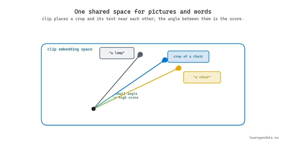
Open vocabulary flips the arrangement. The categories stop living inside the network and start living in a text box you control. So how does a model compare a picture to a word it was never explicitly taught? It puts them in the same room.
This shift did not begin in 3D. It arrived from 2D, where models trained on hundreds of millions of internet images picked up descriptors general enough to transfer almost anywhere. Researchers then found ways to carry those descriptors down onto points.
So the real question is mechanical, not magical. How do you get from a raw cloud to regions you can score against a word, without training a single 3D network? You start by cutting.
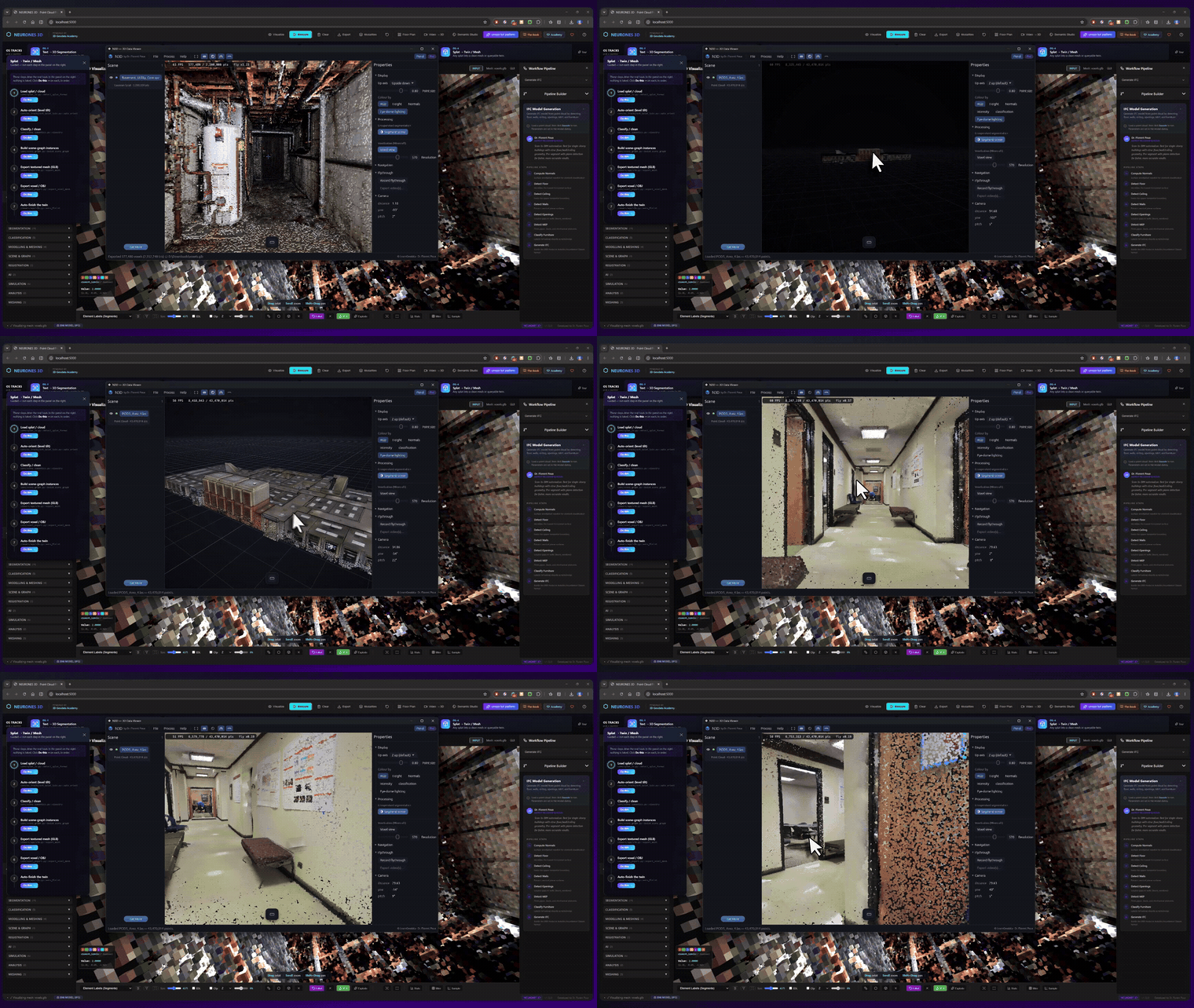
🦚 Florent’s Note: One indoor scan blows past 10 million points before you finish walking the room. Running a foundation model straight on those raw points is a non-starter, it simply chokes. So you render or reuse the source frames, run the 2D model on images, then lift the answer back onto the 3D points. That projection step is where accuracy quietly bleeds, and it is the seam nobody flags until it bites you on a real deliverable.
How Segment Anything Cuts The Scene For You
You cannot name an object you have not isolated first. So the opening move is cutting the scene into parts, and the tool that does this best was never built for 3D at all.
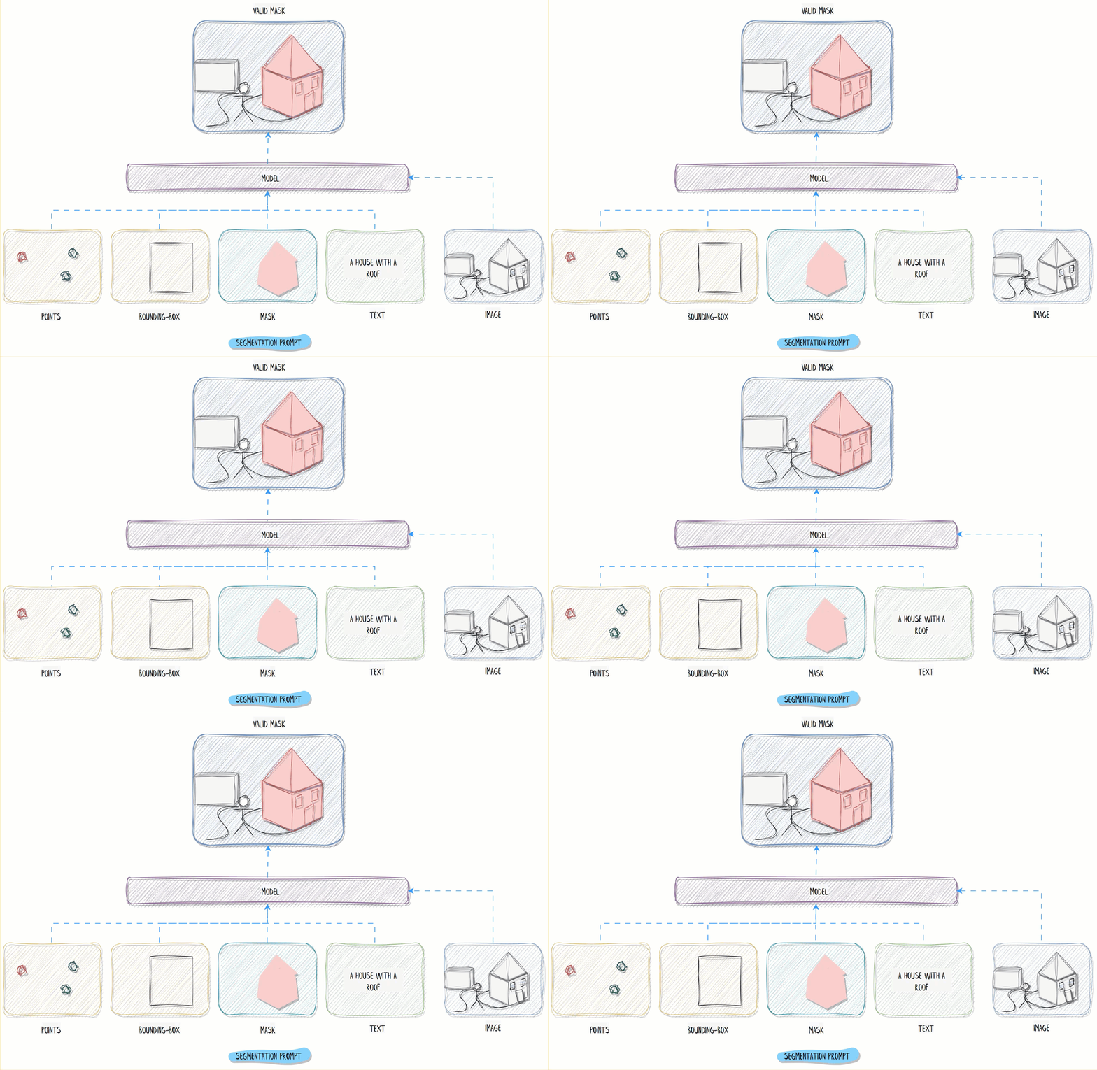
Segment Anything, or SAM, takes an image plus a light prompt (a click, a box) and returns a clean mask around whatever sits there. No category, no fine-tuning on your data, just promptable masks that generalize far past what you would expect. It is the workhorse of the whole stack.
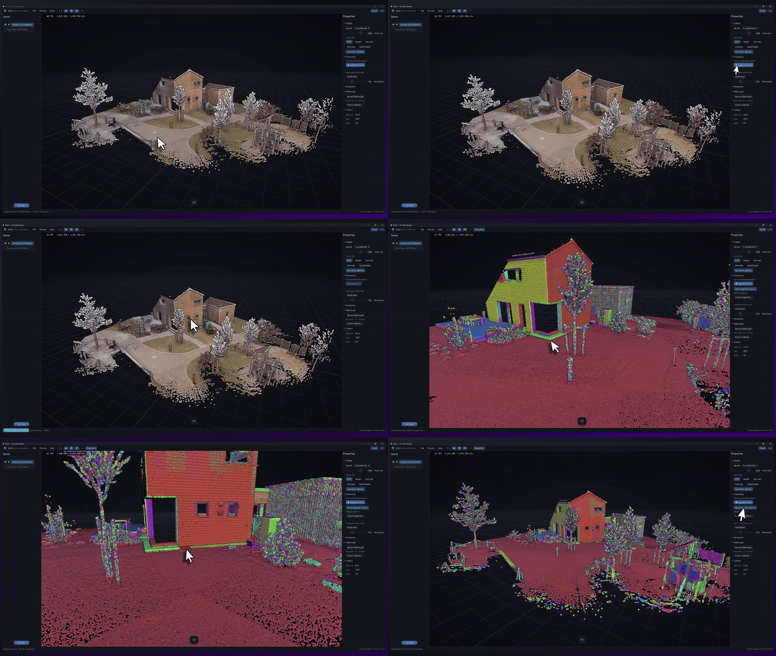
A point cloud is not an image, so you meet SAM where it lives. Render the cloud to a handful of 2D viewpoints, or reuse the RGB frames your reconstruction already saved. Run SAM on each one, then project every mask back onto the points it covers.
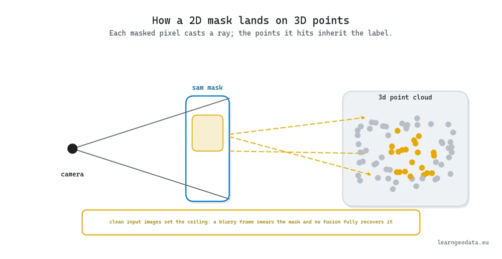
The quality of that back-projection sets your ceiling. Clean, well-exposed source images give SAM crisp boundaries that lift into tight 3D masks. Blurry frames smear them, and no fusion trick downstream fully recovers a bad mask, so if your results look mushy, go look at the pictures before you touch a parameter.
You now have shapes with no names. SAM will happily isolate the lamp and stay perfectly silent about what it is. Closing that gap is the next step, and it is where the typed word finally earns its keep. For the full open-vocabulary 3D semantics method, see our guide to open-vocabulary 3D semantics in Python.
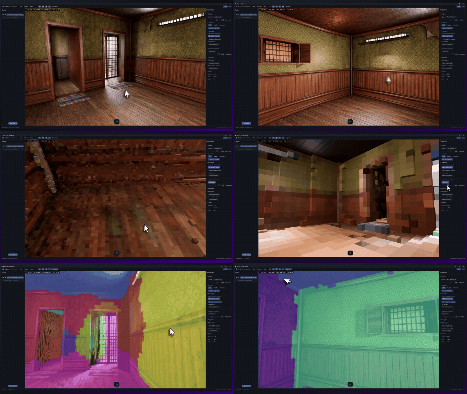
🦥 Geeky Note: The automatic mask generator drops prompts on a regular grid, 32 by 32 out of the box, then prunes overlapping masks by predicted IoU and a stability score near 0.95. Push that grid to 64 by 64 for a cluttered indoor scan and your object count climbs; drop it to 16 by 16 when you need speed. Of every knob SAM exposes, grid density is the one I reach for first, because it moves the result more than the rest combined.
Score Every Region Against Your Word With CLIP
Naming a region with no class list sounds like a trick until you see the mechanism. CLIP learned a single space where a photo of a chair and the string “a chair” land near each other. Embed a masked region, embed your text prompt, take the dot product, and the score tells you how well the word fits.
Swap the word, rerun the dot product, done. There was never a fixed head to edit. That is the beating heart of open-vocabulary 3D segmentation, and stripped down it is a short scoring loop.
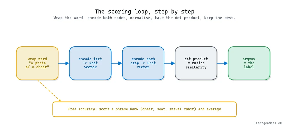
Here is that loop with real libraries, open_clip for the encoder and SAM for the regions. I have folded in the phrase-bank trick from the diagram, because it costs almost nothing and steadies your scores.
import torch, open_clip
from segment_anything import sam_model_registry, SamAutomaticMaskGenerator

# 1. Cut the frame into class-agnostic regions with SAM
sam = sam_model_registry["vit_h"](checkpoint="sam_vit_h_4b8939.pth")
mask_gen = SamAutomaticMaskGenerator(sam, points_per_side=32)
regions = mask_gen.generate(rgb)              # rgb: HxWx3 uint8 image

# 2. One shared space for pictures and words
clip_model, _, preprocess = open_clip.create_model_and_transforms(
    "ViT-B-32", pretrained="laion2b_s34b_b79k")
tokenizer = open_clip.get_tokenizer("ViT-B-32")

@torch.no_grad()
def score_region(rgb, region, phrases):
    # Average a phrase bank into one prototype per class
    tokens = tokenizer([f"a photo of a {p}" for p in phrases])
    t = clip_model.encode_text(tokens)
    t = t / t.norm(dim=-1, keepdim=True)       # unit length
    t = t.mean(dim=0, keepdim=True)
    t = t / t.norm(dim=-1, keepdim=True)
    crop = preprocess(crop_to_mask(rgb, region["segmentation"])).unsqueeze(0)
    v = clip_model.encode_image(crop)
    v = v / v.norm(dim=-1, keepdim=True)
    return float(v @ t.T)                      # cosine similarity

vocab = {"office chair": ["office chair", "swivel chair", "seat"],
         "desk":         ["desk", "table", "workbench"]}
labels = {name: max(score_region(rgb, r, ph) for r in regions)
          for name, ph in vocab.items()}
The line carrying the whole idea is v @ t.T, the dot product of two unit vectors, which is cosine similarity. Notice the caption template too: wrapping your word as “a photo of a {p}” matches how CLIP saw text during training, and that small framing lifts scores by a few points on ambiguous words. The ViT-B-32 weights are a fast default; step up to ViT-L-14 when precision beats latency.
You write crop_to_mask yourself: crop to the region’s bounding box and zero the pixels outside the mask. It is ten lines, and it matters, because a sloppy crop leaks background into the score.
🌱 Growing Note: Prompt design is free accuracy, and the phrase bank in the code above is the cheapest win on offer. Score each region against a handful of phrasings (“office chair”, “swivel chair”, “seat” all point at the same object) and average them. Three phrasings per class trims the wardrobe-versus-cabinet flips noticeably, and it costs you one extra text encode, which is a rounding error next to the image passes.
Fuse Across Views So Your Labels Stop Flickering
CLIP names a region on one frame. Orbit the camera and that same sofa gets scored again, sometimes agreeing with itself, sometimes not. Without a way to say “this patch and that patch are the same object,” your labeled cloud shimmers as you move through it.
Two tools close that gap. DINOv2 turns each frame into a dense grid of self-supervised descriptors, so visually similar patches sit close together and the same object can be matched across frames from a single example. And plain voting handles the rest: once you know an object appears in three views, you tally the labels and let the majority win.
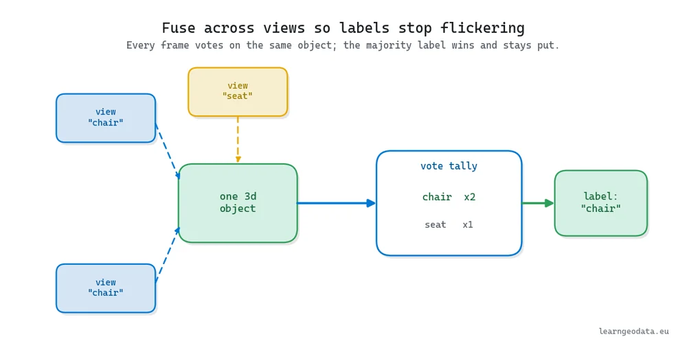
Because DINOv2’s descriptors were learned with no labels at all, they transfer across rooms and objects the network never saw. That is precisely why the trio of SAM, CLIP, and DINOv2 holds together instead of fighting each other for control of the pipeline.
Names from words, matches from examples, consistency from voting. That covers the cases the models get right. But what about the ones they get confidently wrong?
🪐 System Thinking Note: Watch the division of labor, because this pattern repeats all over spatial AI. Each model owns exactly one verb: SAM segments, CLIP names, DINOv2 matches. None was trained on your scene, and none knows the other two exist. The intelligence you ship lives in the wiring you build between them, and that wiring is the part no download replaces, which is also why it is the part worth learning deeply.
Keep The Runner-Ups Because The Score Is Not A Verdict
CLIP hands you a score, not a verdict. “Wardrobe” and “cabinet” can land a hair apart, and a naive argmax picks one with false confidence. That is the honest catch that trips up beginners.
So do not throw away the runner-ups. Keep the top three candidates per region rather than only the winner, because that margin is exactly what a human reviewer needs later. A tight gap is not a failure, it is a flag.
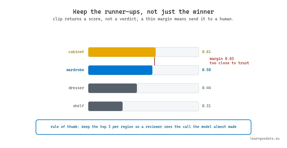
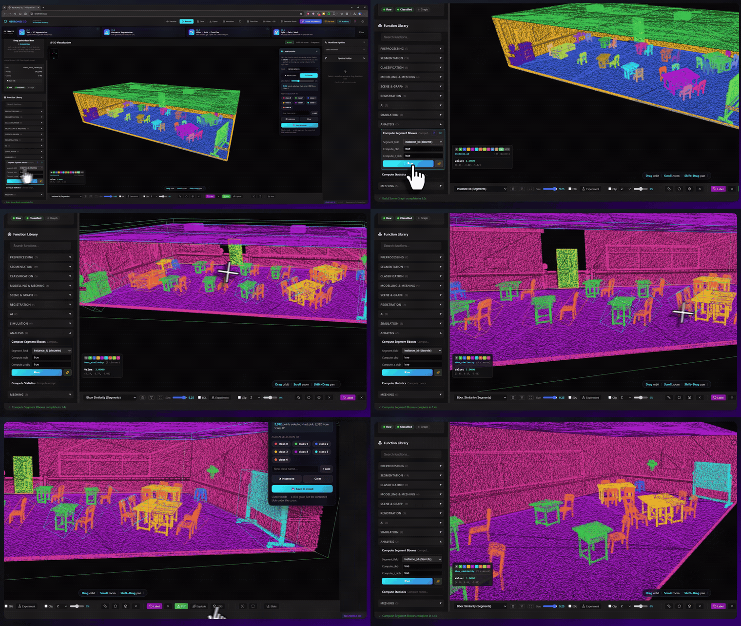
That flag is what makes review affordable. Every region already carries a score, so you auto-accept the confident ones and send only the shaky ones to a human. A well-tuned threshold routes maybe 10 to 15 percent of objects to review, which turns an impossible manual job into twenty focused clicks.
The skill is not the review tool, it is where you spend those clicks. Correct the big ambiguous objects that anchor the scene, and leave the ones the models nailed alone.
🌱 Growing Note: Tune the auto-accept threshold on a scan you have ground truth for, not by feel. Start around a 0.25 cosine score, sweep it upward while you watch how many objects drop into the review pile, and settle where that pile lands near the 10 to 15 percent band. One afternoon of tuning on a known scene buys you a threshold you can reuse across every similar capture after.
🦚 Florent’s Note: Respect the order or pay for it. Masks come out first, the CLIP labels ride on top of them, the review pass cleans those, and only then does the graph get built. I have watched people leap to the shiny end and burn days blaming the model, when a single merged mask three steps back was the actual culprit. Nail 100 clean masks on a scan you know cold before you write one line of graph code.
Turn Named Objects Into A 3D Scene Graph
Clean, named objects are a list, and a room is not a list. The lamp rests on the table, the table faces the sofa, the extinguisher hangs by the door. Those relationships are the difference between a bag of labels and something you can reason about.
A scene graph is how you store them, and it is a plain, strong idea. Nodes are your objects, and edges are the spatial relations between them (on, under, near, supported-by). Once the scene is a graph, it becomes structured knowledge, which is exactly the shape a language model handles well. Our guide to 3D scene graphs with NetworkX and OpenUSD builds one end to end.
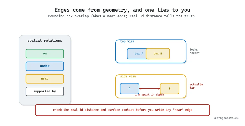
You compute the edges straight from the object geometry. And I want to walk one claim back right here, because it is where people ship bugs.
Feed a clean graph to an LLM and you can ask, in plain English, “what is on the desk nearest the window” or “is there room to set a 40 centimeter box here.” The model reasons over a few dozen typed relations, not over ten million coordinates, because you did the hard work of pulling structure out first.
Tools like NetworkX assemble the graph in a few lines, and the research direction shows up cleanly in OpenScene, which co-embeds 3D points with CLIP descriptors so you can query a whole scene by text. That paper is worth an evening if you want to see where this is heading.
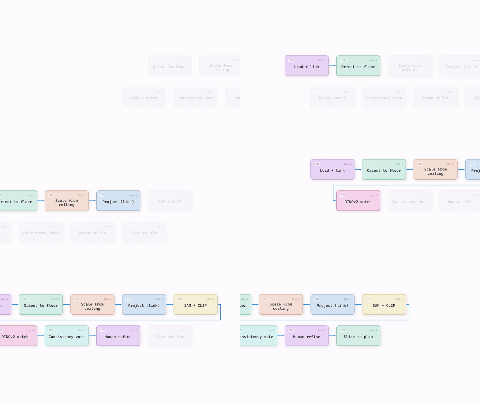
The assembly itself is refreshingly short. You hold each reviewed object as a node carrying its centroid and bounding box, then compute every edge from real 3D geometry instead of a flattened top-down overlap. Here is that graph in a dozen lines.
import numpy as np
import networkx as nx

# objects: one dict per reviewed 3D object
#   {"label": "lamp", "points": (N, 3) float array of its 3d points}
def centroid(o): return o["points"].mean(axis=0)
def bbox(o):     return o["points"].min(0), o["points"].max(0)

def build_scene_graph(objects, near_dist=0.6):
    G = nx.Graph()
    for i, o in enumerate(objects):
        lo, hi = bbox(o)
        G.add_node(i, label=o["label"], center=centroid(o), size=hi - lo)

    for i in range(len(objects)):
        for j in range(i + 1, len(objects)):
            ci, cj = G.nodes[i]["center"], G.nodes[j]["center"]
            d = float(np.linalg.norm(ci - cj))   # true 3d distance, not a projection
            if d > near_dist:
                continue
            dz = ci[2] - cj[2]                    # vertical gap picks the predicate
            rel = "on" if dz > 0.05 else "under" if dz < -0.05 else "near"
            G.add_edge(i, j, relation=rel, distance=round(d, 3))
    return G

graph = build_scene_graph(reviewed_objects)
print(nx.node_link_data(graph))               # serialise the slice, hand it to the LLM
Notice d is a full 3D norm, so two objects that only overlap when seen from above never earn a false “near” edge. That single line is the fix for the depth gotcha the figure above warned about, and it is why you build the graph from geometry rather than from a top view.
🦥 Geeky Note: Trim the graph before it reaches the model. A language model stays sharp across 30 to 50 typed nodes and loses the thread once you hand it thousands of raw relations. So filter down to the objects and edges the current question depends on, then serialize only that slice into the prompt. Small graph in, clean answer out, reliably.
The Open-Vocabulary 3D Segmentation Pitfalls That Cost You A Week
Every failure in this stack has a home, and the fix almost never lives where beginners look for it. When a label comes out wrong, the instinct is to tweak the prompt, when the real bug is three layers down in the masks or the geometry.
So here is the field guide. Match the symptom to the layer, and you stop debugging the wrong thing.
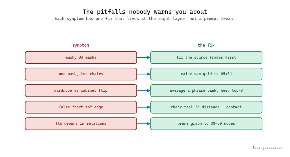
Read that map as a checklist the next time your results look off. Mushy 3D masks send you back to the source frames, not the fusion code, and one mask swallowing two chairs means you raise the SAM grid density. The two that quietly ruin scene graphs are the false “next to” edge (you skipped the 3D distance check) and the drowning LLM (you fed it thousands of relations instead of the fifty that matter). None of these needs a bigger model. They need attention at the right layer.
Where Open-Vocabulary 3D Segmentation Fits In Your Spatial AI Stack
Open-vocabulary 3D segmentation sits at the sharp end of the understand phase in a spatial AI stack, and it only stands up because earlier steps hold it. If you are still cutting clouds into parts by geometry, start with 3D point cloud segmentation and clustering in Python, which is the floor this whole idea rests on.
The descriptors that CLIP and DINOv2 ride on come out of neural networks, so 3D deep learning in Python explains what happens under the hood. After that, meshing your labeled objects into a surface someone can open and measure is the deliver step, covered in 3D data capture, meshing, and visualization with Python. If you want to put a recognition network to work yourself, our step-by-step guide to building a 3D object recognition algorithm walks one build.
If you want the guided version of all of this, with the parameter intuition you cannot get from one article and a path that builds each rung on the last, that is what the 3D AI Program is for. It teaches the wiring between these models as production code, not slides.
Build Your First Open-Vocabulary 3D Segmentation This Week
Reading about this stack will not make it click. Running one rung of it will.
Pick a single scan you already have, or take a thirty-second phone sweep of a room. Get SAM producing masks on one rendered view, open them in Open3D to see the boundaries land on real geometry, and you have your floor. Score those regions against three words you care about, watch the labels fall out, then keep climbing: add the review pass, build the graph, wire the LLM.
If you would rather learn the full path with a hands-on start, the free 3D mission hands you real data and real code to begin. And when you are ready to build the whole stack as a system rather than a demo, the 3D AI Program walks you rung by rung.
So here is the real question: which scan on your drive gets its first mask this week, and what is the first word you will type at it?

Frequently Asked Questions
How Is Open-Vocabulary 3D Segmentation Different From Regular Semantic Segmentation?
Regular semantic segmentation pins you to a class list decided at training time, so anything outside it might as well not exist. The open-vocabulary approach measures each region against free text through a model like CLIP instead, which means a query such as “space heater” works even though no matching label ever appeared during training. The trade-off is a similarity score rather than a hard classification, which is exactly why a review pass earns its place in the pipeline.
Can I Run SAM On A Point Cloud Without A GPU Cluster?
Yes, because Segment Anything runs on 2D images, not on the raw cloud. You render or reuse a handful of views, segment those, then back-project the masks onto the points, so a single consumer GPU handles a room-sized scan comfortably. The lighter ViT-B checkpoint runs faster still if you find yourself memory-bound on a laptop.
How Does CLIP Score A 3D Region Against A Word?
CLIP embeds your masked image crop and your text prompt into one shared space, then a cosine similarity (the dot product of two unit vectors) measures how well the word fits the region. The highest-scoring region wins the label, and swapping the word needs no retraining at all. The open_clip repository ships the pretrained weights and the exact encode functions used in the code above.
Why Do My Scene Graph Edges Get “Near” Wrong?
Edges built from bounding-box overlap alone fail whenever two objects sit close in one projection but far apart in depth. The fix is to check real 3D distance, and where you can surface contact, before you write any relation, and to keep the graph small so the reasoning stays clean. You can build these graphs and the reasoning layer end to end inside the 3D AI Program.
What Python Libraries Do I Need To Start?
You need four things to reach a first result: Open3D to load and view clouds, PyTorch to run the networks, the pretrained SAM and CLIP checkpoints, and NumPy for the geometry math. NetworkX handles the graph assembly at the very end, and no specialized 3D deep-learning framework is required anywhere along the way.

