Here is a frustration you probably know. You scan a room with your phone, the reconstruction looks gorgeous, and then it just sits there. It cannot tell you where the walls are, how many chairs you have, or how big the floor is. This guide fixes that with open-vocabulary 3D semantics: a hands-on Python workflow where pretrained SAM, CLIP, and DINOv2 label, scale, and measure your point cloud, and you train absolutely nothing.
What you’ll learn in this article:
- A nine-step open-vocabulary 3D semantics pipeline you can run end to end, training nothing
- The one idea that makes the hard parts cheap: the pixel-to-point link
- How SAM, CLIP, and DINOv2 each do a different job, and when to reach for which
- The exact parameters that matter, and the failure modes that will bite you
- A small business you could run off the very last step
Estimated reading time: 16 minutes
Why your 3D scans can’t answer a single question (yet)
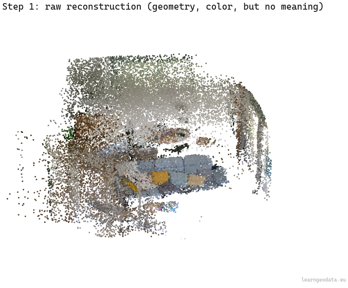
Let me set the scene the way it usually happens. You walk through a room with your phone, filming the way you would to remember where you left something. No rig, no targets, no careful overlap. Five minutes later you have a dense, colorful 3D point cloud, or a 3D Gaussian splat, and it looks fantastic.
Then you try to use it, and it falls flat. Which points are the floor? How many chairs are there? What is the area? The geometry is all there, but the meaning is missing, and meaning is the only thing a machine can act on.
A point cloud without meaning is expensive confetti. The labels are what let it answer a question.
So how do you add that meaning without spending a week clicking labels onto points? Two years ago the answer was “train a segmentation model”. Today it is not. The strong vision models already understand images, and your job is no longer to train one. It is to route what they already know from the picture, where their understanding lives, onto the 3D points, where you actually need it.
And yes, this works well enough for real decisions. As a quick proof: I built a wooden bookshelf for my house straight from one of these scans, took no tape measure to the wall, and it dropped into place.
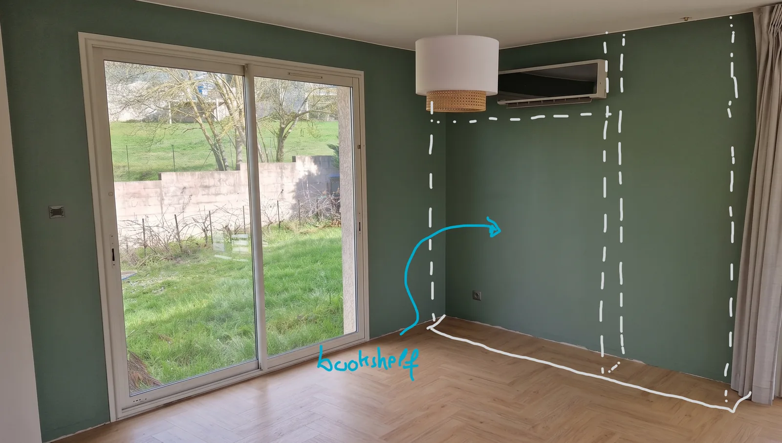
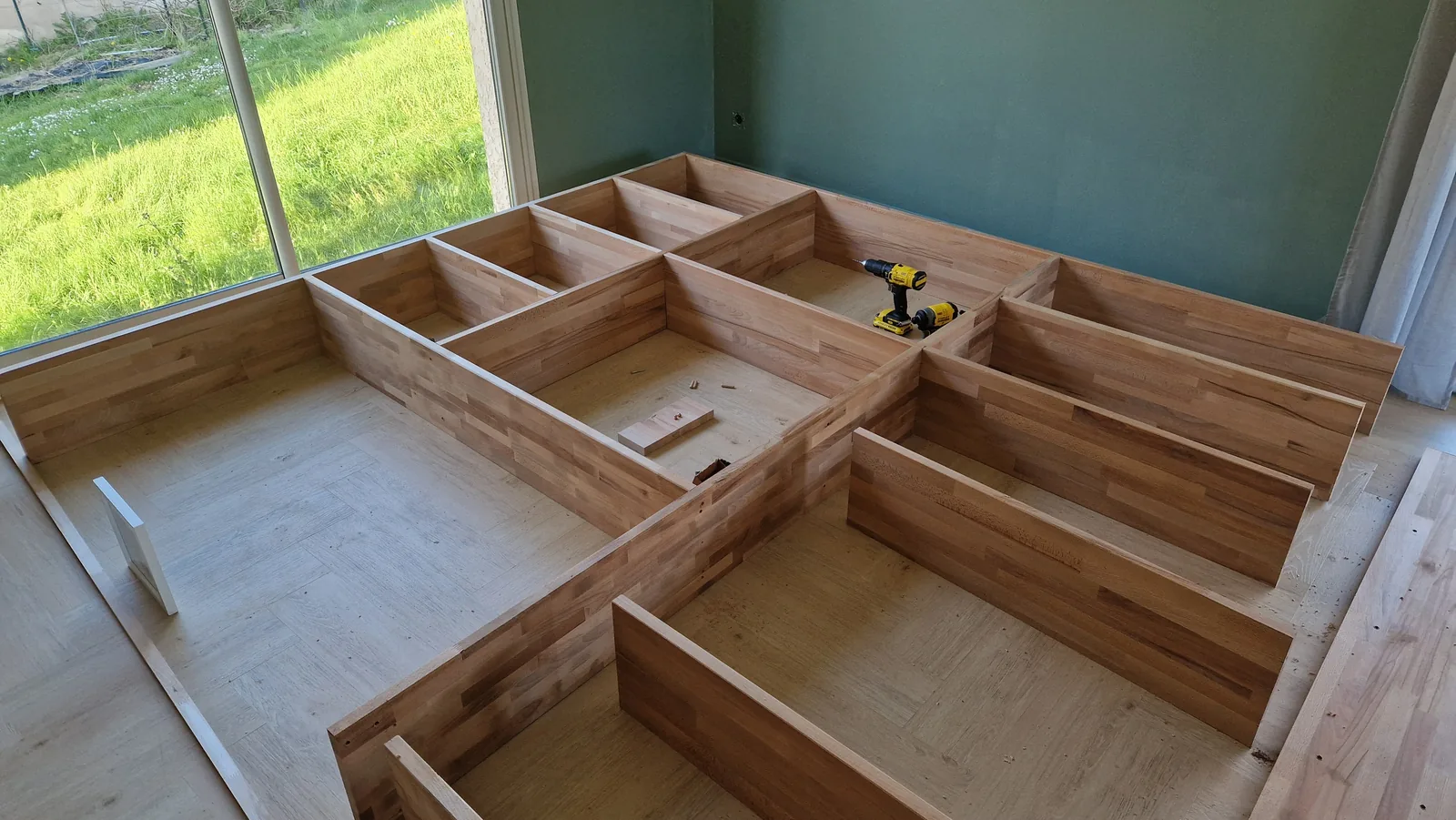
If a machine can understand a room well enough to size furniture for it, the question is no longer “can it understand”, it is “how do you wire that understanding in”.
🦚 Florent’s Note: Quick heads-up before we dig in. This is not a tour of how segmentation works in theory, it is the working skeleton of a real system with the panels taken off. Everything runs in a development mode on plain NumPy and SciPy, so you can watch each stage draw its own figure before you ever load a heavy model or touch a GPU. Read it once top to bottom, then come back and run the functions.
The one idea behind open-vocabulary 3D semantics: the pixel-to-point link
Before the steps, the single concept everything hangs on. Think of it as a Rosetta Stone. That slab mattered because the same text sat there in two languages, so reading one unlocked the other. Your reconstruction has the same gift hiding in it: every 3D point remembers which camera pixel it came from.
Keep that correspondence, and any image model instantly speaks 3D. Run SAM or CLIP or DINOv2 on a flat photo, get a 2D answer, and lifting it onto the cloud is a table lookup, not a fresh re-projection. You paid the geometry cost once, at reconstruction time, and now you collect interest on it forever.
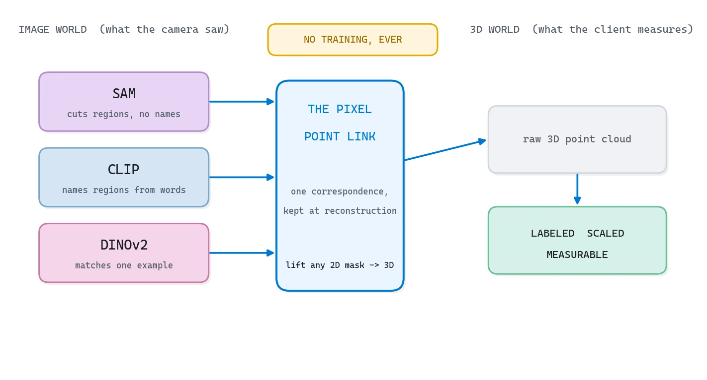
That picture is the whole article in one frame. Protect the link, let the pretrained models do the seeing, and the 3D labels come almost for free. Now let us build it.
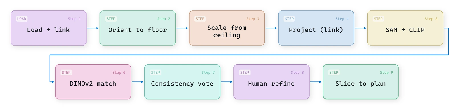
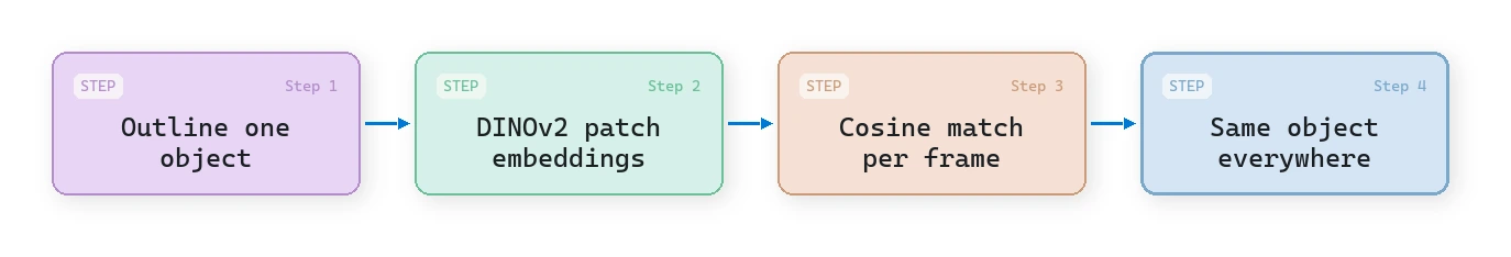
The nine-step open-vocabulary 3D semantics pipeline
I will break the work into nine steps. They are a system, not a checklist: each one exists because the next one leans on it.
- Load the reconstruction and, above all, the pixel-to-point link.
- Orient the cloud to gravity from the floor plane.
- Scale it to real meters from the ceiling.
- Build the projection link with a depth test.
- Propose regions with SAM and name them with CLIP.
- Match one outlined object across every frame with DINOv2.
- Vote across cameras to kill label flicker.
- Put a human in the loop to correct and propagate.
- Slice the result into a measurable floor plan.
Setup: the Python environment and data for 3D semantic segmentation
I want this frictionless. Three things to sort: the environment, the dataset, and the Windows gotchas.
The environment is one conda env. In development mode the pipeline runs on NumPy and SciPy alone, so you read every figure before any model weights enter the picture.
conda create -n spatial_ai python=3.11 -y
conda activate spatial_ai
pip install numpy scipy matplotlib open3d
# Only needed when you wire in the real image models (DEV = False):
pip install torch torchvision transformers
The dataset is the real reconstructed scan you will see throughout, room.ply, roughly 2.2 million points that I subsample to 40,000 for fast iteration. It carries RGB and a per-point class field, and I treat that field as the ground truth the pipeline has to recover. In production this file is whatever your reconstruction engine spits out, co-registered with the processed frames and the camera parameters.
Three Windows traps cost me an afternoon each, so save yourself the trouble. Force UTF-8 on stdout or the figure logs turn to mush under the default code page. Keep the data path plain ASCII, because some point cloud loaders fail silently on accented folder names. And when you move to the real models, write and read the camera JSON as UTF-8 on both machines, or a cross-platform round trip throws on perfectly valid floats.
Which piece holds the rest up? The link. So we start there.
Step 1: Load the reconstruction and the pixel-to-point link
For years I rushed this step, and it cost me every time. You open a point cloud, start processing, and you have already binned the most valuable thing in the file.
A reconstruction is not one object, it is three: the geometry, the frames the camera saw, and the provenance tying each point back to its exact source pixel. The first two are obvious. The third is the one that makes everything after it cheap, and it is the one people throw away.
def load_scene():
    """Return a scene dict: xyz, rgb, labels, frames metadata, provenance link."""
    if not DEV:
        sys.path.insert(0, NEURONES_3D)
        from core import scene_semantics, pixel_projection  # noqa: F401
        scene = scene_semantics.load_scene(DATA_FILE)
        # In prod the provenance .npz is written by the reconstruction engine.
        return scene

    # DEV: load the real labeled scan; its labels are the answer we recover.
    c = dv.load_cloud(DATA_FILE, max_points=40000, want_labels=True)
    xyz = c["xyz"].astype(np.float32)
    rgb = c["rgb"]
    labels = c["labels"] if c["labels"] is not None else np.zeros(len(xyz), int)

    # Synthesize camera frames around the scene and the pixel-point provenance.
    img_h, img_w = 540, 960
    K = np.array([[700, 0, img_w / 2], [0, 700, img_h / 2], [0, 0, 1]], float)
    n_frames = 6
    frames, cams = [], []
    center = xyz.mean(axis=0)
    radius = float(np.linalg.norm(xyz.max(0) - xyz.min(0))) * 0.6
    for f in range(n_frames):
        ang = 2 * np.pi * f / n_frames
        pos = center + radius * np.array([np.cos(ang), np.sin(ang), 0.25])
        fwd = center - pos
        fwd /= np.linalg.norm(fwd)
        right = np.cross(fwd, [0, 0, 1]); right /= np.linalg.norm(right)
        up = np.cross(right, fwd)
        R = np.stack([right, -up, fwd])           # world -> camera
        frames.append((img_h, img_w))
        cams.append({"frame": f, "R": R, "position": pos, "intrinsic": K})

    return {"xyz": xyz, "rgb": rgb, "labels": labels, "frames": frames,
            "cams": cams, "K": K, "img_shape": (img_h, img_w),
            "names": _class_names(labels), "n_points": len(xyz)}
Watch the camera convention, because it decides whether Step 4 works. I store R as a world-to-camera rotation and position as the camera center in world coordinates, which pairs cleanly with the projection math later. The ring of six synthetic cameras is just a stand-in so the geometry has something real to chew on in development. In production those come from structure-from-motion on the keyframes, and the provenance ships as a compact array: for each point, which frame and which pixel. Keep that array and you never solve correspondence again.
🦚 Florent’s Note: I learned this the expensive way. My early pipelines tossed the link and rebuilt it at query time with depth maps. It worked, it was slow, and it drifted. The day I started saving the link at reconstruction time, half my “segmentation bugs” turned out to be registration bugs I could finally see and fix.
We have geometry. It is also upside down. So orientation comes first, and here is why.
Step 2: Orient the point cloud to gravity with RANSAC
A fresh reconstruction lands in an arbitrary frame, and ours arrives tilted and flipped. You could nudge it straight by hand with a gizmo, but that does not scale. The data already knows which way is up: the floor is the most reliable horizontal surface in any indoor scan, so recover gravity from it.
I fit the dominant near-horizontal plane with RANSAC, then rotate the whole cloud so that plane’s normal points straight up. One robust estimate, no fiddling.
def fit_plane_ransac(pts, thresh=0.03, iters=300):
    """Return (normal, d, inlier_mask) for n.x + d = 0, the largest plane found."""
    best_inliers, best_n, best_d = None, None, None
    n_pts = len(pts)
    for _ in range(iters):
        i, j, k = RNG.choice(n_pts, size=3, replace=False)
        v1, v2 = pts[j] - pts[i], pts[k] - pts[i]
        nrm = np.cross(v1, v2)
        norm = np.linalg.norm(nrm)
        if norm < 1e-8:
            continue
        nrm = nrm / norm
        d = -nrm @ pts[i]
        dist = np.abs(pts @ nrm + d)
        inliers = dist < thresh
        if best_inliers is None or inliers.sum() > best_inliers.sum():
            best_inliers, best_n, best_d = inliers, nrm, d
    return best_n, best_d, best_inliers
Two numbers drive this. The inlier threshold (thresh=0.03, three centimeters before scaling) sets how thick a plane you accept; keep it just above the cloud’s noise floor so a slightly bumpy floor still reads as one plane. The iteration count (iters=300) is your odds of drawing three points that all sit on the floor. Push the threshold too high and a sloped ceiling sneaks into the floor’s inliers, and your whole gravity vector leans.
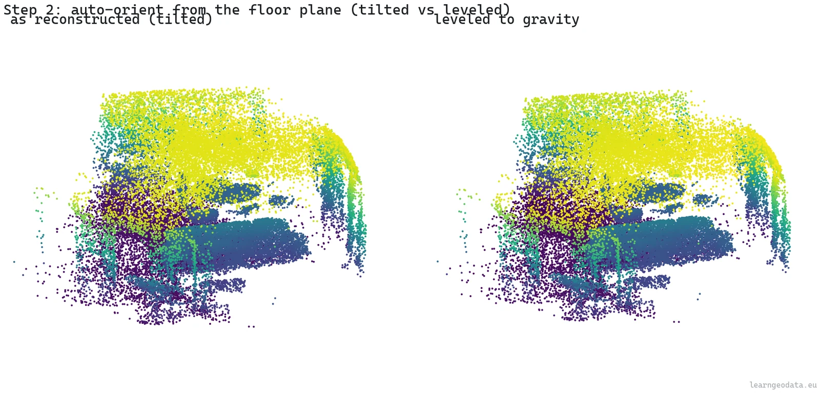
🦥 Geeky Note: I draw the RANSAC triples from the lowest 35 percent of Z, not the whole cloud. That one trick lifts the odds of a clean floor hit enough that I can keep iterations low and still land a stable normal. The production engine goes further, merging parallel planes before it solves a small frame correction, but this single-plane core already gives you 90 percent of the win.
The tilt here is barely a degree, which sounds like nothing until you remember that the scale, the slice height, and the floor-versus-wall split all assume Z really points up. The room is level now, but it has no size. A reconstruction from images has no idea whether it captured a dollhouse or a cathedral. So how do we hand it meters?
Step 3: Scale the point cloud to real meters
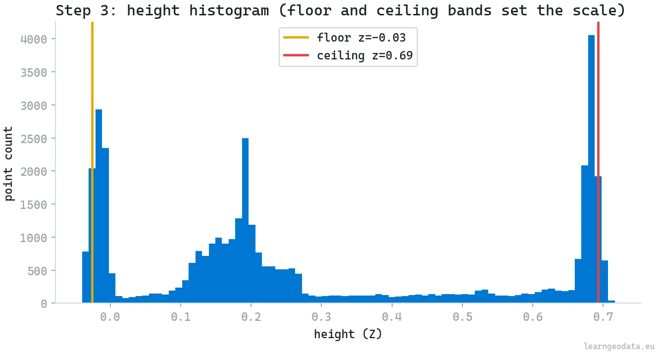
Reconstructions from monocular video or structure-from-motion are scale-free. To make the cloud metric you need exactly one known distance, and indoors the ceiling volunteers it for free. Floor and ceiling each show up as a dense band in the height histogram, and the gap between them is the room height. Tell the system the ceiling sits near 2.5 meters and the whole scene snaps to real units.
def identify_and_scale(scene):
    """Detect the floor/ceiling bands, scale the scene so ceiling = reference."""
    if not DEV:
        sys.path.insert(0, NEURONES_3D)
        from core import scene_inventory, scene_transform
        scene = scene_inventory.identify(scene)
        return scene_transform.apply_scale(scene, CEILING_REFERENCE_M)

    z = scene["xyz"][:, 2]
    hist, edges = np.histogram(z, bins=80)
    centers = 0.5 * (edges[:-1] + edges[1:])
    dense = centers[hist > 0.25 * hist.max()]
    floor_z, ceil_z = float(dense.min()), float(dense.max())
    measured_height = ceil_z - floor_z
    scale = CEILING_REFERENCE_M / measured_height if measured_height > 1e-6 else 1.0

    scene["xyz"] = (scene["xyz"] * scale).astype(np.float32)
    scene["scale"] = scale
    scene["room_type"] = "indoor room"
    return scene
The knob to watch is the density threshold (hist > 0.25 * hist.max()). Floor and ceiling are the two most crowded horizontal slabs in nearly any room, so a quarter of the peak height isolates them cleanly while the sparse furniture in between gets ignored.
The honest weakness is that hard-coded 2.5 meters. Fine for a living room, wrong for a cellar or a warehouse, which is exactly why I flag it rather than hide it.
🌱 Growing Note: Swap the constant for a learned prior. Run a tiny room-type classifier on the cloud, or just ask a vision-language model “what room is this?” on a single frame, then look up a typical ceiling height: office 2.7 meters, cellar 2.2, retail 3.5. Now the scale is data-driven, and the same pipeline sizes a basement and a showroom correctly.
We have a level, metric room. Time to make the link concrete and start moving information from the photos onto the points.
Step 4: Project the link with a depth test
This is the step that earns back the whole design. For each frame I project every point into the camera, then keep a per-pixel nearest-depth buffer so a point glimpsed through a closer surface does not steal that surface’s label. The output, per frame, is the set of visible points and their pixel coordinates. After that, lifting any mask is trivial: take the mask’s true pixels, look up the points sitting behind them.
def project_points_to_frame(cam, img_shape, points, depth_tol=0.04):
    """Return (visible_idx, uv) for points landing inside this frame, front-surface only."""
    H, W = img_shape
    R = np.asarray(cam["R"], float)
    pos = np.asarray(cam["position"], float)
    K = np.asarray(cam["intrinsic"], float)
    Pc = (points - pos) @ R.T                     # world -> camera
    z = Pc[:, 2]
    front = z > 1e-6
    zf = np.where(front, z, 1.0)
    u = np.round(K[0, 0] * Pc[:, 0] / zf + K[0, 2]).astype(np.int64)
    v = np.round(K[1, 1] * Pc[:, 1] / zf + K[1, 2]).astype(np.int64)
    inb = front & (u >= 0) & (u < W) & (v >= 0) & (v < H)
    idx = np.flatnonzero(inb)
    if idx.size == 0:
        return idx, np.empty((0, 2), np.int64)
    zbuf = np.full((H, W), np.inf)
    np.minimum.at(zbuf, (v[idx], u[idx]), z[idx])
    keep = z[idx] <= zbuf[v[idx], u[idx]] * (1.0 + depth_tol) + 1e-6
    idx = idx[keep]
    return idx, np.stack([u[idx], v[idx]], axis=1)
The parameter that earns its place is the depth tolerance (depth_tol=0.04, four percent). Drop it and a point on a far wall seen through a doorway inherits the doorframe’s label, and your sofa smears onto the curtains behind it.
Four percent holds the front surface and drops the background bleed, and I tune it per scan: tighter for clean tripod captures, looser for shaky handheld ones where the depth estimate wobbles. The np.minimum.at call builds the z-buffer in a single vectorized pass, which is why this runs in milliseconds even across six views.
🦥 Geeky Note: Notice there is no pixel loop anywhere. The projection, the bounds check, the z-buffer scatter, all of it is array math. On a 40,000 point cloud the per-frame cost is dominated by that one scatter into the buffer. This is the difference between a link you rebuild without thinking and one you avoid because it is slow.
The link is live. Time to let the pretrained models loose. How do you label a cloud without labeling a single point by hand?
Step 5: Label the cloud with SAM and CLIP (open vocabulary)
Two pretrained models do all the work in this step, and I train neither. SAM, the Segment Anything Model, slices each frame into regions without knowing what any of them are, like cutting a picture into puzzle pieces. CLIP then scores each piece against a list of words you type in plain text and keeps the best match. “Open vocabulary” just means that word list is a string you can rewrite between runs, which is the whole point of open-vocabulary 3D semantics: the labels are words, not a frozen model head.
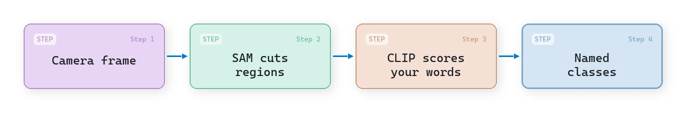
The two models split the labor cleanly. SAM answers “where are the boundaries?” and never names anything, so it happily handles objects it was never told about. CLIP answers “which of these words fits this region?” by dropping the cropped region and your candidate words into one shared space and grabbing the nearest match. Neither saw your room in training, and you can change the word list (“sofa, radiator, skirting board”) between runs without retraining a thing. If you want this running end to end on real scans, it is the backbone of the academy’s Segment Anything for 3D course.
def propose_and_label_segments(scene):
    """Return per-point class ids from SAM proposals + CLIP open-vocab naming."""
    if not DEV:
        sys.path.insert(0, NEURONES_3D)
        from core import cloud_open_vocab
        return cloud_open_vocab.label_cloud_openvocab(
            scene["xyz"], scene["rgb"], scene["link"], prompts=list(scene["names"].values()))

    gt = scene["labels"]
    noisy = gt.copy()
    flip = RNG.random(len(gt)) < 0.12               # 12% per-point flicker
    noisy[flip] = RNG.integers(0, gt.max() + 1, size=int(flip.sum()))
    scene["labels_noisy"] = noisy
    return noisy
In development I stand in for the model output with the scan’s own segments and then deliberately corrupt 12 percent of the point labels, because that noise is exactly what Step 7 has to clean up. The number is not arbitrary. It is close to the cross-frame disagreement a real open-vocabulary labeler produces on a handheld scan, where the same point gets confidently different names from different angles. Testing the cleanup on perfect labels would just be lying to myself about whether it works.
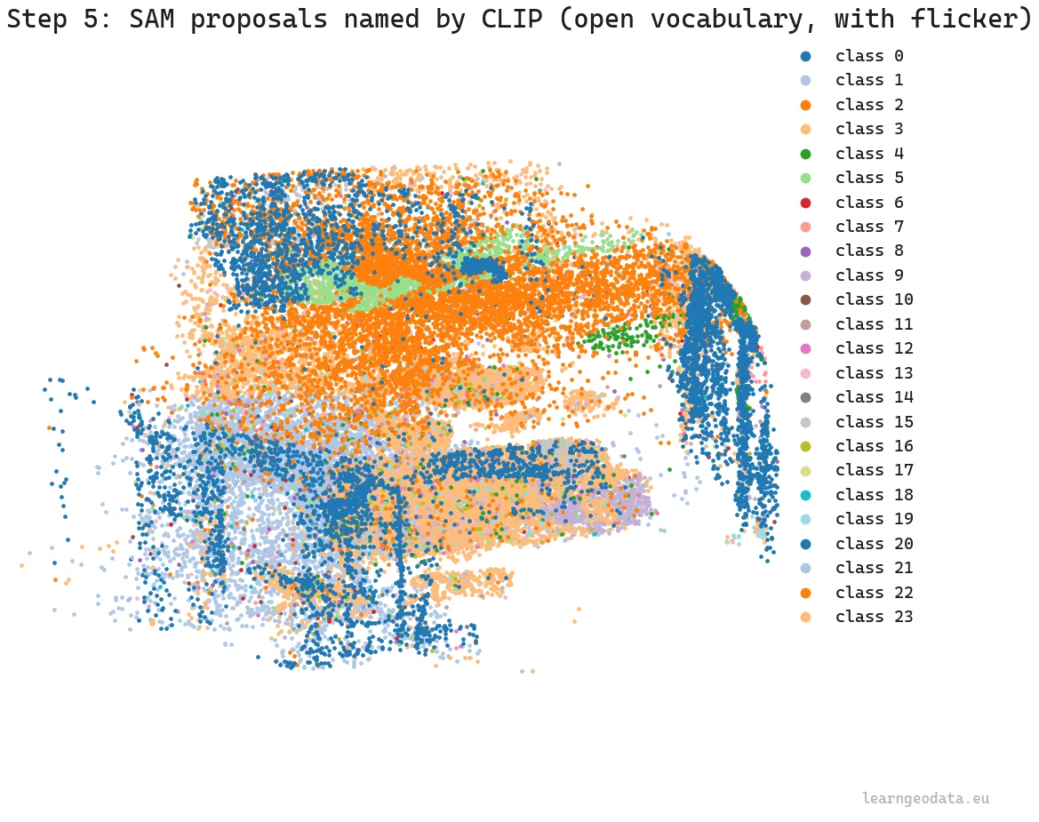
🦚 Florent’s Note: The first time I ran SAM and CLIP on a real scan, I braced for the naming to be the hard part. It was not. The hard part was that every camera had its own opinion, and the cloud shimmered between classes as I orbited it. The labels were good. The agreement was the problem, and that single realization reshaped the entire back half of this pipeline.
Words are powerful, but sometimes you do not have a word, you have an example. What if pointing at one object found it everywhere?
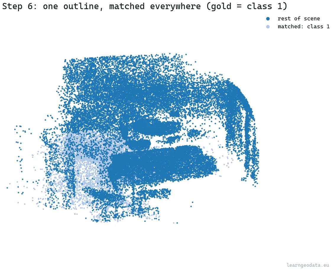
Step 6: Match one object across frames with DINOv2
This is the cleverest move in the workflow, so it is worth slowing down. You outline a single object in one frame, a rough lasso, and DINOv2 finds that same object in every other frame. No class name, no training, no examples beyond the one you drew.
It runs on patch embeddings. DINOv2 turns a frame into a grid of embedding vectors, one per patch. The production trick is to subtract the positional part of those embeddings first, so similarity is driven by what a patch looks like, not where it sits. Then it averages the foreground patches you outlined into a prototype and cosine-matches that prototype across each target frame.
The point is that you never define what a “sofa” is. You hand it one example, and because DINOv2’s self-supervised features place visually similar patches close together, the same object lights up across every other frame on its own. That is the in-context trick: one demonstration instead of a class name or a training set.
def incontext_match(scene, target_class=TARGET_CLASS):
    """Find one outlined object across frames, lift the match to 3D point indices."""
    if not DEV:
        sys.path.insert(0, NEURONES_3D)
        from core import incontext_seg
        refs = scene["reference_outlines"]          # [(image, mask), ...]
        return incontext_seg.propagate(refs, scene["frames_dict"], image_size=768, tau=0.6)

    gt = scene["labels"]
    link = scene["link"]
    target_pts = set(np.flatnonzero(gt == target_class).tolist())
    matched = np.zeros(len(gt), bool)
    for fid, fr in link.items():
        vis = fr["idx"]
        is_target = np.array([int(i) in target_pts for i in vis])
        keep = is_target & (RNG.random(len(vis)) < 0.90)   # 90% per-frame recall
        matched[vis[keep]] = True

    scene["matched_target"] = matched
    return matched
The numbers that matter live in the production call. The working image size is 768 pixels, rounded to the patch grid, because smaller loses the object and larger burns compute on a phone frame for nothing. The merge threshold tau=0.6 decides how eagerly nearby patches cluster into one match, and 0.6 is the sweet spot where a sofa stays one object instead of shattering into cushions. In development I model each frame as 90 percent recall, then union the lifts across all six frames, which recovers nearly the whole object even though no single view sees all of it. That union across views, which only the link makes possible, is the quiet hero of the whole thing.
🦥 Geeky Note: DINO came out of a finding that still delights me: a vision transformer trained with no labels at all learns to segment objects on its own, its attention maps just light up on the foreground. DINOv2 scaled that up. The in-context use here, one example then find the rest, is the same instinct as a kid learning a new word from a single point of the finger. The DINOv2 paper and the official code are both open.
So now we have labels from two routes, words and examples. They disagree across cameras. How do we stop the cloud from shimmering?
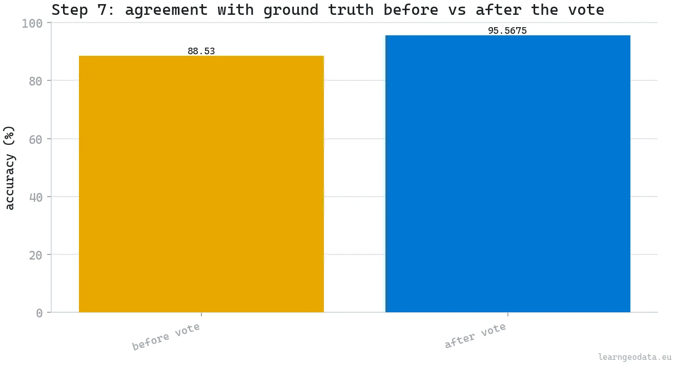
Step 7: Fix 3D label flicker with a geometry vote
Here is the problem nobody warns you about. One point reads “wall” from camera A and “window” from camera B. Across a full scan the cloud flickers, and a flickering cloud breaks everything downstream, from a 3D scene graph to a client report. The fix is a vote, and crucially the vote is settled by geometry, not by whichever camera shouted last.
def spatial_consistency_vote(scene, labels, k=16, min_cluster=20):
    """Return labels after a k-NN majority vote that resolves cross-camera flicker."""
    if not DEV:
        sys.path.insert(0, NEURONES_3D)
        from core import semantic_refine
        cleaned, _ = semantic_refine.segment_consistency_refine(
            scene["xyz"], labels, list(scene["names"].values()),
            min_cluster=min_cluster, normal_angle_deg=12.0, k=k)
        return cleaned

    from scipy.spatial import cKDTree
    xyz = scene["xyz"]
    tree = cKDTree(xyz)
    _, nn = tree.query(xyz, k=k, workers=-1)        # (n, k) neighbor indices
    C = int(labels.max()) + 1
    neigh_labels = labels[nn]                       # (n, k)
    counts = np.zeros((len(xyz), C), np.int32)
    for j in range(neigh_labels.shape[1]):
        counts[np.arange(len(xyz)), neigh_labels[:, j]] += 1
    voted = counts.argmax(axis=1).astype(np.int32)
    return voted
The neighbor count (k=16) sets how much local context each point listens to. Too few and a genuine thin feature gets shouted down by its surroundings; too many and you blur the boundaries between objects. Sixteen is a solid default for indoor density.
🪐 System Thinking Note: Structure and objects are different kinds of things and want different rules. A floor is planar, so you grow it with a normal-similarity gate (a cosine around 12 degrees) that refuses to cross a sharp edge. A chair is not planar, so that same gate would shatter it, and you group it by plain Euclidean connectivity instead. The one-line vote above kills most of the flicker, but it is this structure-versus-object split that turns “demo” into “production”.
The vote handles the bulk. Automation always frays at the edges, though. Where exactly should a human step in?
Step 8: Human-in-the-loop 3D labeling that scales
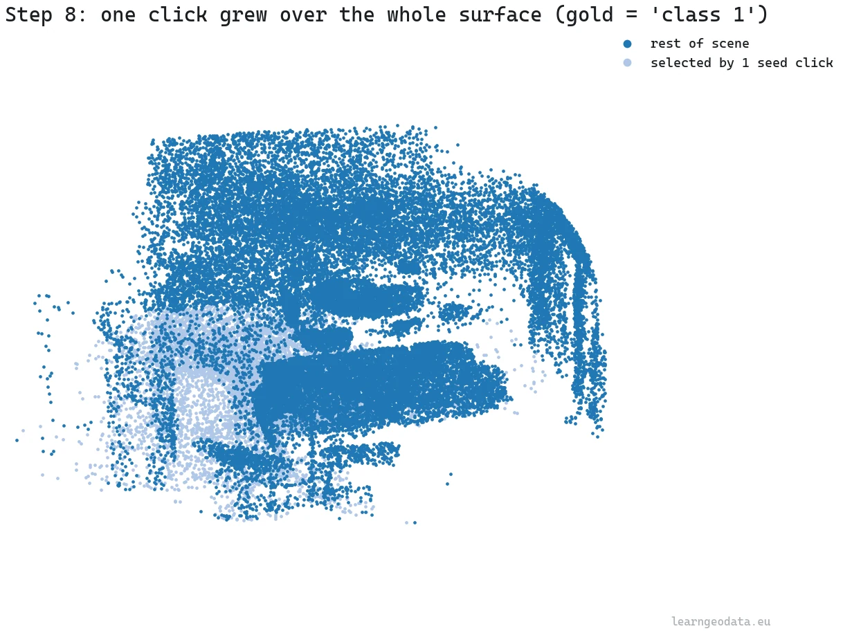
Let me say the unfashionable thing out loud: the human is not the weak link here, the human is the quality gate. The goal was never zero humans, it is humans spent only where judgment beats compute. And the interaction is tiny. Click one point, say “this is floor”, and the system grows that label across the connected surface and stops at the boundaries. One click reclaims an entire plane.
def human_refine(scene, labels, seed_class=0, n_seeds=1):
    """Region-grow a corrected label from a seed point. Returns updated labels."""
    if not DEV:
        sys.path.insert(0, NEURONES_3D)
        from core import semantic_refine
        out, _ = semantic_refine.seed_propagate(
            scene["xyz"], labels, list(scene["names"].values()),
            seeds=scene["user_seeds"])
        return out

    from scipy.spatial import cKDTree
    xyz = scene["xyz"]
    gt = scene["labels"]
    seed_class = int(np.bincount(gt).argmax())

    tree = cKDTree(xyz)
    _, nn = tree.query(xyz, k=12, workers=-1)        # (n, 12)

    cls_idx = np.flatnonzero(gt == seed_class)
    centroid = xyz[cls_idx].mean(axis=0)
    seed = int(cls_idx[np.argmin(np.linalg.norm(xyz[cls_idx] - centroid, axis=1))])

    region = np.zeros(len(xyz), bool)
    region[seed] = True
    frontier = [seed]
    while frontier:
        cur = frontier.pop()
        for nb in nn[cur]:
            if not region[nb] and gt[nb] == seed_class:
                region[nb] = True
                frontier.append(int(nb))

    out = labels.copy()
    out[region] = seed_class
    return out
The growth walks a k-nearest-neighbor graph (k=12), so the flood fill only hops between points that already agree, and it is fast because the graph is built once. In one run a single interior click spread across more than eight thousand connected points and swept up the mislabeled ones along the way.
That is the leverage: the human supplies one bit of intent, the geometry supplies the extent. In production the growth radius is derived from local point spacing (three times the median nearest-neighbor distance), so the same click behaves on a dense indoor scan and a sparse outdoor one. The real skill, and it is a skill, is choosing where to click: spend your clicks on the big ambiguous planes that move accuracy the most, not on the easy stuff the models already nailed. I go deeper on this human-in-the-loop workflow, where to click and why, in a dedicated walkthrough on 3D point cloud labeling in Python, and teach it at production scale in the academy’s applied semantic segmentation course.
We have a clean, labeled, scaled scene. Now the part the client actually asked for: something they can measure.
Step 9: Export a measurable floor plan from the point cloud
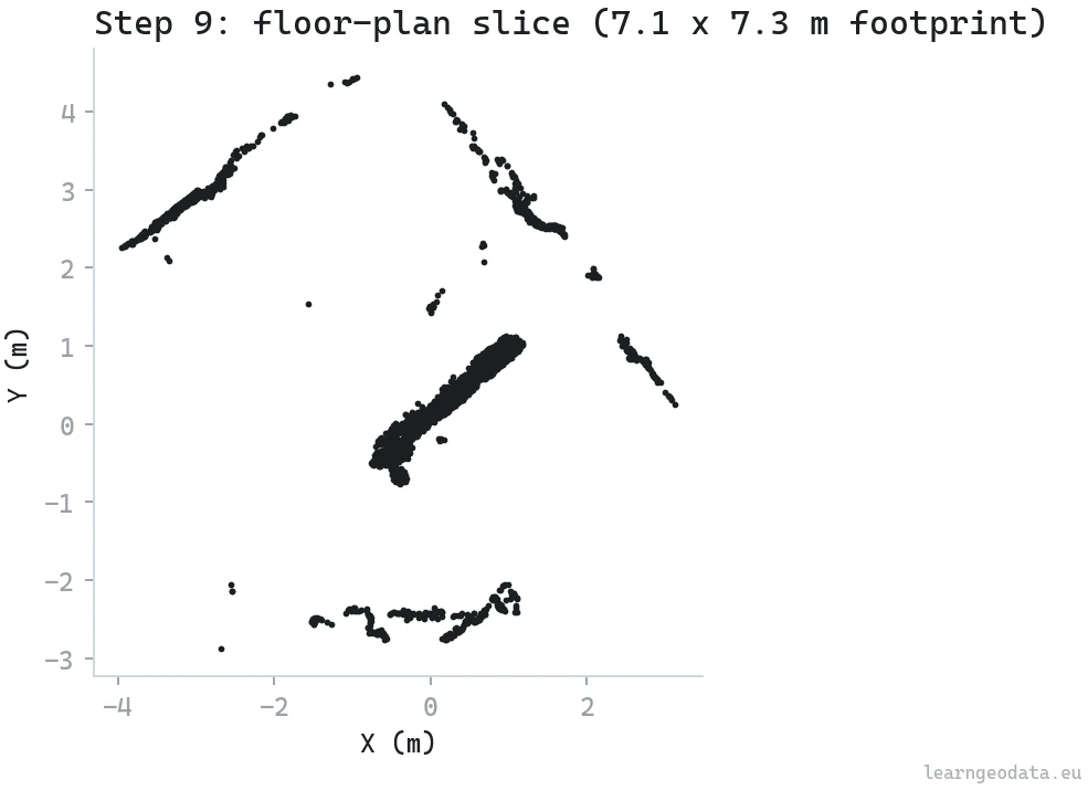
Most clients do not want a point cloud, they want a plan they can read dimensions off. So take a horizontal slab a few hundred millimeters thick at a sensible cut height, drop the Z, and you have a section. Its XY extent is the room’s footprint in meters, straight from the cloud, with no CAD redraw and no tape measure in the room.
def export_floorplan_slice(scene, thickness_m=0.30, out_path=None):
    """Cut a horizontal slab, report the footprint, write a slice cloud."""
    if not DEV:
        sys.path.insert(0, NEURONES_3D)
        from core import slice_export
        return slice_export.export_slice(scene, thickness=thickness_m)

    xyz = scene["xyz"]
    z = xyz[:, 2]
    cut = float(np.percentile(z, 5)) + 1.0
    slab = (z >= cut - thickness_m / 2) & (z <= cut + thickness_m / 2)
    pts2d = xyz[slab][:, :2]
    if out_path is None:
        out_path = os.path.join(os.path.dirname(os.path.abspath(__file__)),
                                "floorplan_slice_dev.ply")
    ext_x = float(pts2d[:, 0].max() - pts2d[:, 0].min()) if len(pts2d) else 0.0
    ext_y = float(pts2d[:, 1].max() - pts2d[:, 1].min()) if len(pts2d) else 0.0

    with open(out_path, "w", encoding="utf-8") as f:
        f.write("ply\nformat ascii 1.0\n")
        f.write(f"element vertex {len(pts2d)}\n")
        f.write("property float x\nproperty float y\nproperty float z\nend_header\n")
        for x, y in pts2d:
            f.write(f"{x:.4f} {y:.4f} {cut:.4f}\n")
    return out_path
Two choices run this: the cut height (one meter above the fifth-percentile floor) and the slab thickness (thickness_m=0.30). A meter up is the standard architectural cut, above the furniture clutter but through the walls and door openings. Thirty centimeters is thick enough to catch sparse walls in a noisy cloud and thin enough that you read one clean line instead of a smear.
🦥 Geeky Note: One caution worth stating plainly. The plan inherits the capture’s scale error. A careless handheld sweep is fine for a renovation sketch and risky for as-built tolerances. I will show dimensions off these slices, but I will not certify them off a phone capture, and neither should you.
🌱 Growing Note: There is a genuine service hiding in this last step. Walk a space with a phone, run this pipeline, and ship a dimensioned floor plan plus a labeled model the same day, for properties that would never justify a survey crew. Real estate listings, insurance pre-assessments, small renovation quotes. The capture is free and the deliverable is what a client pays for, so the margin lives entirely in the orchestration you just learned.
From script to product: where AI coding agents fit
Let me be blunt about where the value actually sits. This script is the domain core: the link, the vote, the human gate, the parameter choices. That is the part fifteen years of doing this taught me, and it is the part an AI cannot invent for you. But wrapping it into a usable tool, a desktop app with a 3D viewport, an outline brush, an export dialog, is exactly what an AI coding agent is great at.
So the division of labor is honest. You are the orchestrator: you decide that the depth tolerance loosens on noisy captures, that the human should click the big ambiguous planes first, that the ceiling prior should depend on room type. The agent is the builder: it turns those calls into a thousand lines of UI and glue while you watch. I built the production version exactly this way, holding the design decisions and letting the agent handle the boilerplate. That is not laziness, it is playing to each side’s strengths. I wrote up that split, the human holding the architecture while the agent writes the glue, in a founder’s blueprint for 3D pipeline architecture.
Where open-vocabulary 3D semantics breaks (and how to ship anyway)
Step back and look at what nine small functions pulled off together. A careless phone video became a level, metric, labeled 3D room, with one object matched across every frame, a flicker-free cloud, and a measurable floor plan. Nothing was trained. The compounding is the whole story: each step was cheap because the last one set it up, and the link from Step 1 paid for the lift in Step 6 and the slice in Step 9.
Now the part that will save you a bad afternoon, because trusting this blindly will burn you.
The link is only as good as the registration. A reprojection error of a couple of pixels bleeds labels across object boundaries, and no amount of voting fully recovers from a bad pose graph. Open-vocabulary matching stumbles on rare categories that CLIP and DINOv2 barely saw in training, and on transparent or reflective surfaces where the image itself lies about the geometry. The consistency vote can confidently propagate a wrong majority in a region where every camera agreed and every camera was wrong. And the floor-plan numbers inherit the capture’s scale error, full stop.
So verify on a held-out subset before you trust any of this at scale, and keep the human on the high-stakes calls. The system is strong precisely because it knows what it cannot do alone.
Zoom out and the pattern is bigger than one pipeline. The cost of understanding is falling toward zero while the cost of judgment holds steady. The models will keep getting better at naming and matching. What stays scarce is knowing which correspondence to protect, which prior to encode, which click to make.
🪐 System Thinking Note: My bet for the next two years: this moves from “label a scan” to “query a scan”. Once the link is standard and the semantics are reliable, the cloud becomes a database you ask questions of, and then an interface an agent acts through. The open-vocabulary 3D semantics pipeline here is the unglamorous plumbing under that future, and plumbing is where reliability lives.
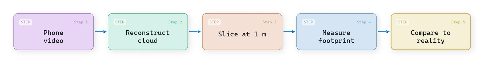
Build your first open-vocabulary 3D pipeline this week
Reading is not the thing that makes this click. Doing it once is.
So pick a room you already know the size of. Take a thirty-second phone video of it, reconstruct it, and slice it.
Then compare the footprint your slice reports against the real dimensions you can measure with a tape.
That single loop, capture to measurement, will teach you more about where this technology genuinely helps and where it quietly lies than any article ever could.
Do that, and you will have run a complete open-vocabulary 3D semantics pipeline on your own data. Then come build the rest.
Resources for open-vocabulary 3D semantic segmentation
- The DINOv2 paper and its official code, for the self-supervised embeddings behind the in-context matching.
- The Segment Anything (SAM) paper, for the class-agnostic proposal model.
- The CLIP paper, for open-vocabulary naming from plain text.
- Open3D, the library I lean on for point cloud I/O and geometry.
- On this site: Segment Anything for 3D, applied semantic segmentation, and a hands-on 3D point cloud labeling in Python walkthrough.
- The 3D Geodata Academy, where I teach this orchestration end to end with production code and real human-in-the-loop labeling.
Keep going with spatial AI
If this pipeline is the kind of thing that excites you, the 3D Geodata Academy has a deep stack of free content to get you started, and when you are serious about building a real business around spatial AI, the 3D AI Architect program is the most complete thing I have ever designed for it.
I’m Florent Poux, Ph.D. I research and teach spatial AI, and I wrote 3D Data Science with Python (O’Reilly). I spend my days turning research into systems that ship, and my goal here is to hand you the foundations the strong models cannot replace.
Frequently asked questions about open-vocabulary 3D semantics
Can I do open-vocabulary 3D semantics without training a model?
Yes. SAM proposes regions, CLIP names them from text, and DINOv2 matches examples, all pretrained. The work is orchestration and lifting masks to 3D through the pixel-point link, not training.
How do you lift a 2D mask onto a 3D point cloud?
You keep a link from each point to the frame and pixel it came from, then a mask’s true pixels look up the points behind them, with a depth test so background seen through the mask is not mislabeled.
Why does my labeled point cloud flicker between classes?
Different cameras label the same point differently. A geometry-based vote over k nearest neighbors, ideally with a structure-versus-object split, replaces per-point flicker with per-segment consensus.
How do you scale a point cloud from a video to real meters?
Reconstructions from images are scale-free. Detect the floor and ceiling as dense height bands and set their gap to a known reference, around 2.5 meters indoors, to make the scene metric.
Is a phone-video floor plan accurate enough to build from?
For renovation sketches and rough quotes, yes. For as-built tolerances, no, because the plan inherits the capture’s scale error. Keep a human on high-stakes measurements.

