

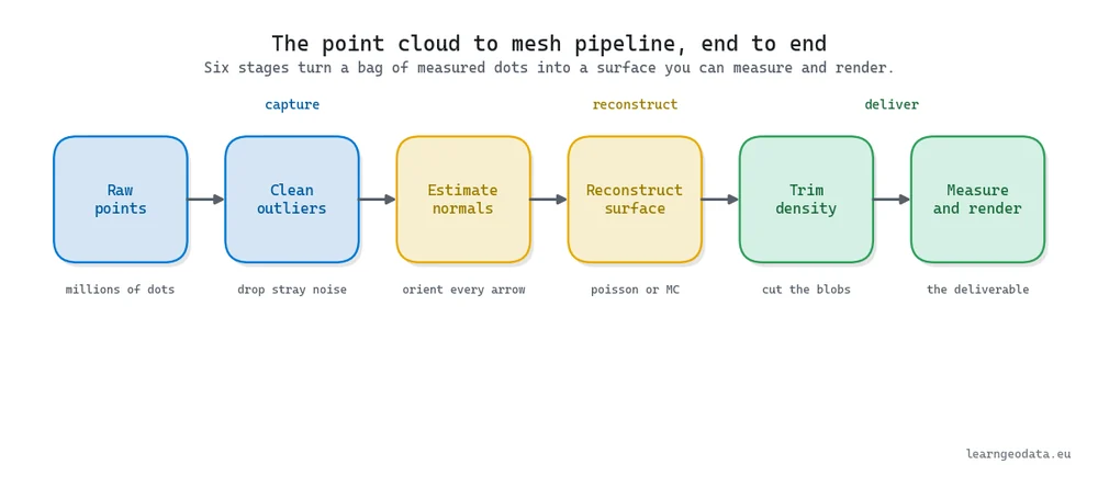
Point cloud to mesh conversion adds connectivity to raw coordinates: it decides which three points form a triangle, so a swarm of dots becomes a surface you can measure. In Python you clean the cloud, estimate and orient normals with Open3D, run Poisson reconstruction, then trim the low-density blobs Poisson invents.
A few million colored dots snap into place. Then the client asks for the floor area.
| What it is | Turning a point cloud into a mesh: adding the connectivity that says which three points form a triangle, so the data gains an inside, an outside, and dimensions you can measure |
| What you build | An Open3D pipeline that orients normals, runs Poisson reconstruction at depth 9, trims the lowest-density 3 to 4 percent of vertices, then renders the result and compares two scans |
| Libraries | Open3D and NumPy for the pipeline, plus Potree, CloudCompare and Blender for viewing, inspection and batch rendering |
| Worked on | Synthetic rooms you generate in a dozen lines of NumPy, and building captures running to tens of millions of points |
| Level | Beginner to intermediate. Assumes Python, and you need no scanner to follow along. |
Here is the path this guide takes, so you can jump straight to the part you need:
- What Point Cloud to Mesh Conversion Really Means
- The Sensor Decides Your Noise Floor First
- Picking A Capture Method That Fits The Job
- Debugging Your Pipeline With Synthetic Point Clouds
- Estimate Normals, The Step You Cannot Skip
- Run Poisson Reconstruction In Open3D
- Trim The Blobs Poisson Invents
- Marching Cubes Or Poisson For Point Cloud To Mesh
- Ball Pivoting When You Want The Real Points
- Reading Change Between Two Point Clouds
- Rendering Millions Of Points Without Choking
- Common Point Cloud To Mesh Pitfalls
- Where This Fits In The Wider 3D Spatial AI Workflow
- Your First Point Cloud To Mesh This Week
- Frequently Asked Questions
That gap is the whole reason this guide exists. Going from point cloud to mesh is the step where a swarm of measured dots turns into a real surface with an inside, an outside, and dimensions you can defend in a meeting. And the good news is that Python does the entire job with free, open tools.
What you’ll learn in this article:
- Why the sensor you pick sets your accuracy ceiling long before you write a line of Python
- The one Open3D call you cannot skip, and what happens to your surface when you do
- How to run Poisson reconstruction and read the depth dial without blowing up your memory
- How to compare two scans and turn the difference into a change map you can trust
- How to keep tens of millions of points interactive on an ordinary laptop
Estimated reading time: 14 minutes
What Point Cloud to Mesh Conversion Really Means
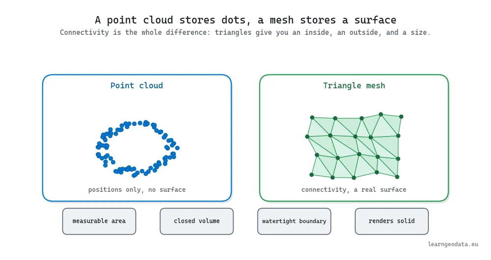
Point cloud to mesh conversion starts from an honest limitation nobody mentions when they hand you a scanner. A point cloud is only coordinates. Three numbers per dot, sometimes a color, and nothing that says point A and point B sit on the same wall.
So there is no area, no volume, and no watertight boundary. It looks solid on screen and behaves like fog the second you try to measure it.
A mesh closes that gap by adding connectivity. It decides which three points form a triangle, and all at once you have a skin instead of a swarm. That single addition is what lets you compute a floor area, print the object, or hand a stakeholder something that reads as real.
So the work ahead is a chain, and every link can quietly poison the next one. Capture sets your noise, meshing amplifies whatever survived, and visualization exposes all of it at full resolution. You get clean results by knowing which link is weakest, not by buying a pricier scanner, so let me start where the data is born.
The Sensor Decides Your Noise Floor First
Every dot in your cloud is a physical measurement, and how it was measured decides how much you can trust it. A time-of-flight scanner clocks how long a laser pulse takes to bounce back. A structured-light sensor projects a known pattern and reads how the surface warps it. A photogrammetry rig emits nothing and instead triangulates depth from the parallax between overlapping photos.
Why does this land on your meshing later? Because a surface rebuilt from a shaky phone capture wants completely different handling than one from a survey scanner. And if you do not know which one you are holding, you’ll spend a day blaming your reconstruction code for errors the sensor baked in.
So read the physics well enough to predict your noise floor before you touch the data, not after a failed mesh. Our guide to 3D sensor types, active versus passive lays out how each family behaves.
🦥 Geeky Note: Time-of-flight is a brutal timing problem. Light travels roughly 0.3 meters every nanosecond, so 1 mm of range accuracy means resolving the return pulse to about 3 picoseconds. That is why affordable indoor depth cameras dodge raw pulse timing and lean on phase shift or a projected pattern, trading absolute range for a cheaper clock.
Picking A Capture Method That Fits The Job
Knowing the sensor families is not the same as knowing what to rent on Monday. There is a real distance between “structured light exists” and the call to send up a drone, roll out a terrestrial scanner, or just walk a room with a phone.
The decision comes down to three things: scale, budget, and the accuracy you’ll have to defend when someone questions your deliverable six months later. A drone with a LiDAR payload maps an open quarry in a single flight. A handheld SLAM unit is faster indoors but drifts on long corridors, and a careful photogrammetry setup can rival either one if you control lighting and keep enough frame overlap.
Each of these choices caps the quality of your final mesh before a single point exists.
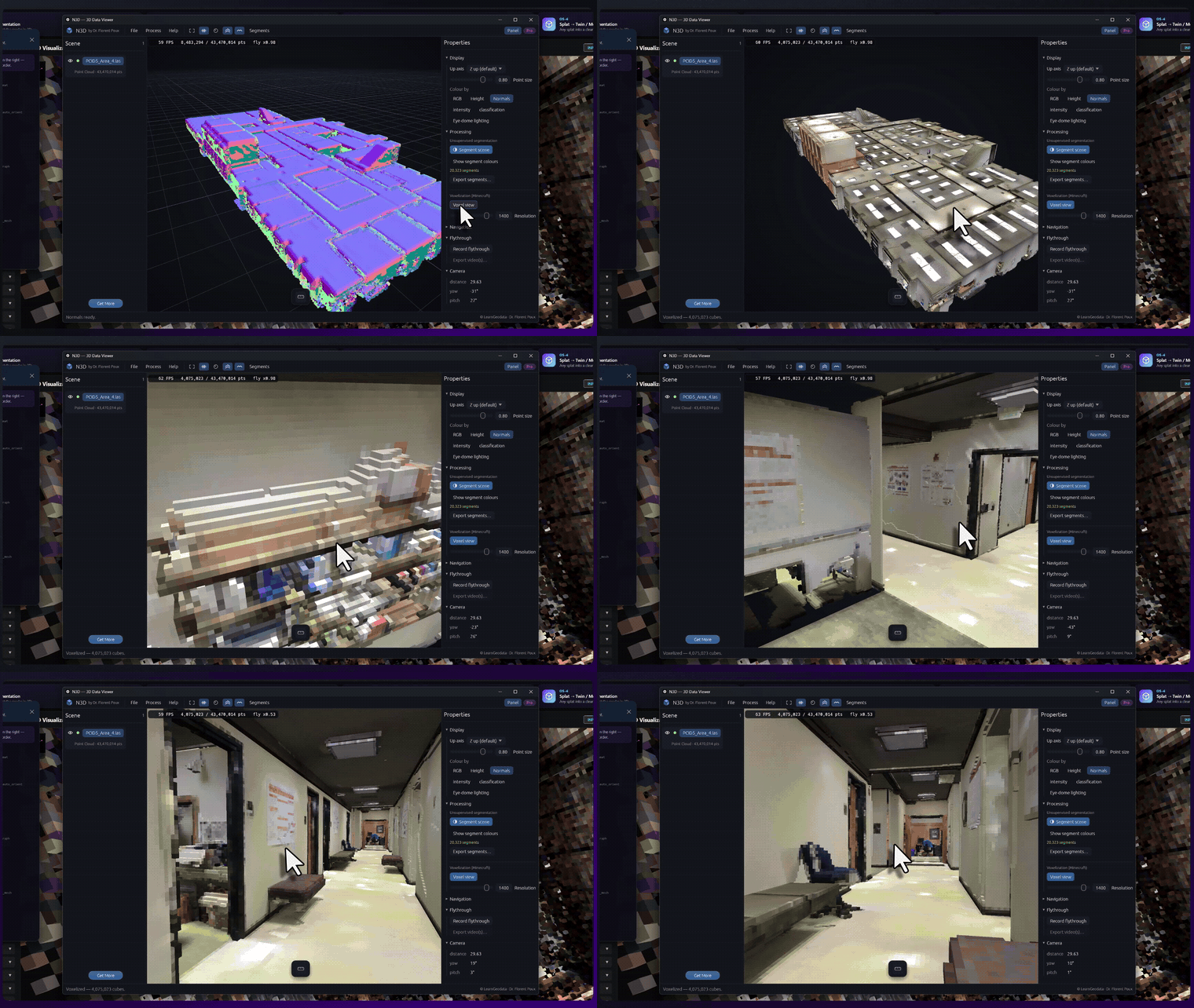
🦚 Florent’s Note: Picture a stone church facade, roughly 18 meters tall. Fly it with a drone and you get the roofline and upper tracery no ground scanner can reach, but the lower carvings come back soft. Walk the base with a terrestrial scanner and those carvings turn crisp while the roof falls into shadow. On jobs like that I stop arguing which tool wins and fuse both clouds, because the honest answer is that the deliverable needs a bit of each.
Debugging Your Pipeline With Synthetic Point Clouds
Synthetic point clouds save beginners weeks of debugging. You do not need a scanner to build and test your meshing code at all.
You can write a dozen lines of Python that place walls, a floor, and some furniture as points, and because you generated the scene, you already know where every surface belongs. That known truth is gold. When the answer key lives in the same script, every error you see belongs to your reconstruction, not to some invisible calibration quirk in a black-box device.
Want to know how your Poisson surface reacts to 3 percent positional noise? Add exactly 3 percent and watch it deform. Our tutorial on synthetic point cloud generation of rooms shows how to build these scenes from scratch.
🌱 Growing Note: Do not treat synthetic data as training wheels you outgrow. When you move into 3D deep learning later, procedurally generated scenes with perfect labels become a serious tool, because hand-labeling real clouds is slow and expensive. A generator that emits a fresh labeled room every second is a data pipeline, not a toy.
Estimate Normals, The Step You Cannot Skip
Now the core conversion, and the place people rush and then regret. Before any reconstruction runs, you need normals.

A normal is the little arrow that says which way a patch of surface faces, and Poisson cannot run without consistent ones. Here is the trap: estimating a normal gives you a direction, but the sign stays ambiguous, so half your arrows can point inward. Leave them that way and the reconstruction folds the surface back through itself, handing you a mesh with the topology of a paper bag someone sat on.
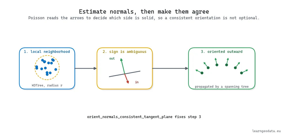
So the sequence is not a style choice. You estimate normals from local neighborhoods first, then run a separate call that walks the cloud and forces every normal into agreement, usually along a minimum spanning tree. Skip that second call and the depth dial you are about to meet cannot save you.
Let me show the core in Open3D, because once the normals are handled the reconstruction is genuinely short.
Run Poisson Reconstruction In Open3D
Two algorithms do the heavy lifting in this field, and they reason in opposite directions. Marching Cubes, from Lorensen and Cline’s 1987 paper, drops a 3D grid over your data and, cube by cube, decides where the surface slices through each cell. Poisson reconstruction, from Kazhdan’s 2006 work, treats your oriented points as samples of a smooth field and solves for the single watertight surface whose gradient best fits them.
Poisson is the one you’ll reach for again and again on scanned surfaces, so here is the full recipe end to end. Notice how short the reconstruction itself is once normals are in order.
import numpy as np
import open3d as o3d

# Load a cleaned cloud (outliers already removed)
cloud = o3d.io.read_point_cloud("facade.ply")

# 1. Estimate normals from each point's local neighborhood
cloud.estimate_normals(
    search_param=o3d.geometry.KDTreeSearchParamHybrid(radius=0.06, max_nn=32)
)

# 2. Force every normal into a consistent inside/outside direction
cloud.orient_normals_consistent_tangent_plane(k=25)

# 3. Poisson: depth is the resolution dial (higher = finer + more memory)
mesh, densities = o3d.geometry.TriangleMesh.create_from_point_cloud_poisson(
    cloud, depth=9
)

# 4. Trim the low-density skin Poisson invents where you never scanned
densities = np.asarray(densities)
keep = densities > np.quantile(densities, 0.035)
mesh = mesh.remove_vertices_by_mask(~keep)
The single argument worth building intuition around is depth. It sets the resolution of the octree Poisson solves on, so depth 8 gives a fast, chunky preview and depth 11 gives fine detail at a steep memory cost.
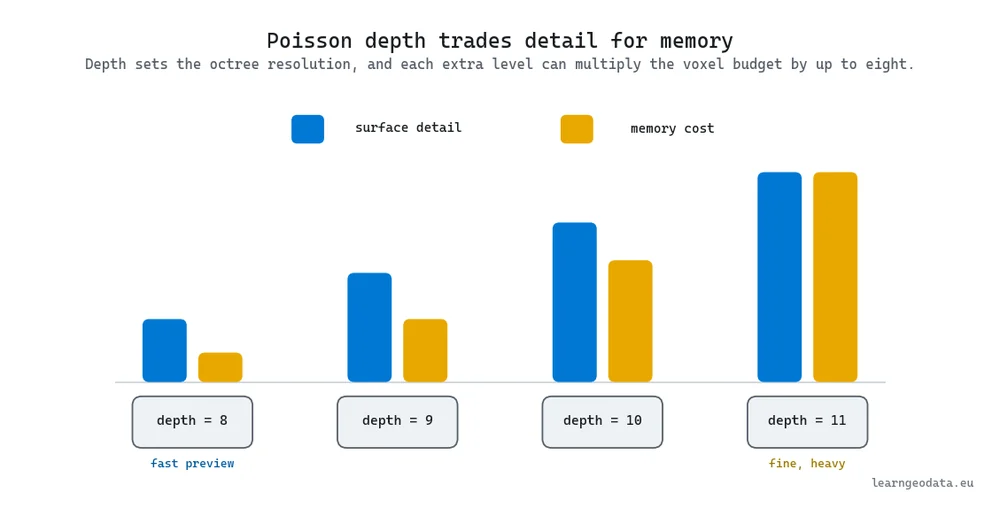
And the ordering in that code is load-bearing. Because create_from_point_cloud_poisson reads the normals to decide which side of each patch is solid, calling it before orient_normals_consistent_tangent_plane gives you a confident, watertight, completely wrong surface.
🦥 Geeky Note: Poisson’s memory scales with that octree depth, and it scales fast. Each extra level of depth can multiply the voxel budget by up to eight, so jumping from depth 9 to depth 11 is not “a bit more detail”, it can be dozens of times the memory. Preview at depth 8, and commit to depth 10 or 11 only once your normals and cleanup hold up.
Trim The Blobs Poisson Invents
Poisson invents blobs, and that is the one predictable side effect you have to plan for. Because it always returns a closed surface, it invents geometry in the regions you never scanned, sealing the shape with thin balloons and webbing near the boundaries.
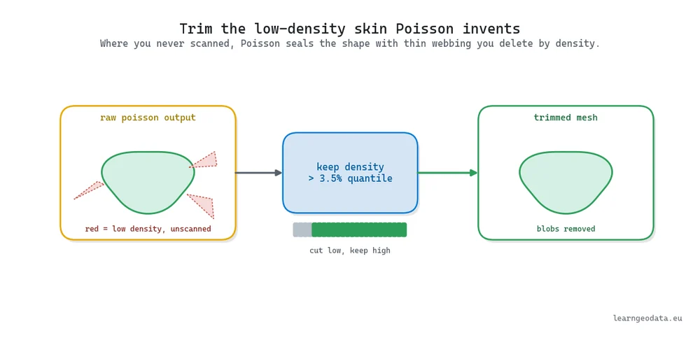
The fix is already in the code above. Poisson hands back a per-vertex density value alongside the mesh, and those low-density vertices are exactly the invented ones. Cut the bottom 3 to 4 percent by density and the balloons drop away while your real surface stays intact.
So think of it as two moves, not one: reconstruct to get a watertight shape, then trim by density. Skip the trim and every hole in your scan becomes a bubble in your deliverable.
🪐 System Thinking Note: Meshing is a lossy compression step, and naming it that changes how you treat it. You discard the exact point positions and keep a triangulated approximation, so the real question is not “is it watertight” but “did I keep the detail that matters and drop the noise that does not”. The normal radius (here 0.06 m) and the Poisson depth are where you set that trade, which is why you tune them per scan instead of hunting for one magic setting.
Marching Cubes Or Poisson For Point Cloud To Mesh
Choosing between Marching Cubes and Poisson comes down to where your data already lives. Poisson for scanned surfaces where you want a smooth, closed skin, and Marching Cubes when your data already lives on a grid or a volume, like a medical scan or a signed-distance field.
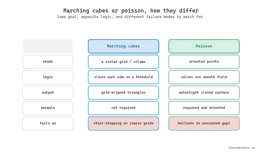
Their failure modes tell you when you have picked wrong. Marching Cubes on a coarse grid gives you visible stair-stepping, a blocky surface that betrays the cell size. Poisson on a cloud with holes gives you those bubbles, confident geometry where no data ever existed.
Both are decades old, both are open, and both ship inside Open3D. So the real skill is reading your data and picking the logic that matches it, not memorizing the API. Our tutorial on building a 3D mesh from a point cloud with marching cubes walks that algorithm in full.
Ball Pivoting When You Want The Real Points
Ball pivoting is the third reconstruction worth knowing, and it makes the opposite trade to Poisson. Poisson fits a smooth field and hands you a watertight skin that no longer passes through your exact measurements. Ball pivoting keeps every measured point as a mesh vertex and simply connects them, so sharp edges stay sharp and nothing gets rounded off.
Picture a small ball rolling across the surface of your cloud. Wherever it rests on three points without falling through, those three become a triangle. It reads the same normals you already estimated, so the recipe drops right in after the orientation step.

import numpy as np
import open3d as o3d

# Load the cloud and give it the same oriented normals Poisson needs
cloud = o3d.io.read_point_cloud("facade.ply")
cloud.estimate_normals(
    search_param=o3d.geometry.KDTreeSearchParamHybrid(radius=0.06, max_nn=32)
)
cloud.orient_normals_consistent_tangent_plane(k=25)

# Size the rolling ball from the cloud's own point spacing
distances = cloud.compute_nearest_neighbor_distance()
avg = np.mean(distances)
radii = [1.5 * avg, 3.0 * avg]  # two ball sizes catch fine and coarse spacing

# Ball pivoting keeps your measured points as the mesh vertices
mesh = o3d.geometry.TriangleMesh.create_from_point_cloud_ball_pivoting(
    cloud, o3d.utility.DoubleVector(radii)
)

# Save the surface, then take a quick look in the Open3D viewer
o3d.io.write_triangle_mesh("facade_bpa.ply", mesh)
o3d.visualization.draw_geometries([mesh])
The radii list is the dial here, the way depth is for Poisson. Set the ball too small and it drops through every gap, leaving a mesh full of holes. Set it too large and it bridges over detail you wanted to keep.
The honest part is what ball pivoting refuses to do. Because it only ever connects points you actually measured, it never invents a bubble to seal an unscanned region, but it also will not close a hole your scan never covered. So reach for Poisson when you need a smooth, watertight shell, and reach for ball pivoting when you would rather see an honest gap than a confident guess.
Reading Change Between Two Point Clouds
One scan is a snapshot. The value often shows up when you capture the same place twice and ask what moved.
Scan a construction site this month and next, or a cliff face before and after a storm, and the signal is the difference between the two clouds. The make-or-break step is registration: getting both scans into one shared coordinate frame before you subtract anything.
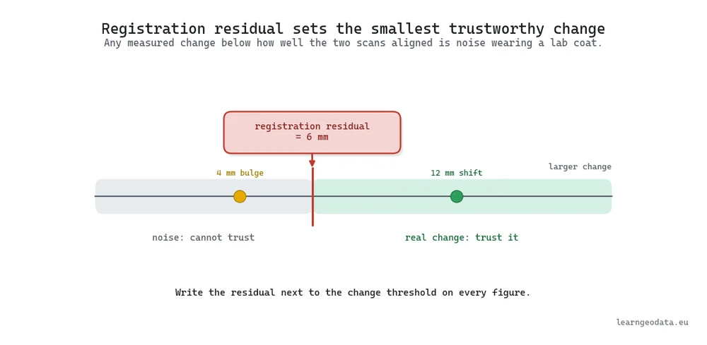
Once the two epochs lock together, the per-point distance becomes a clean heatmap, and that heatmap is frequently the actual product the client is paying for. But there is a floor under it. If your two scans only aligned to 6 mm, any 4 mm “change” you get excited about is alignment slop wearing a lab coat.
🦚 Florent’s Note: I’ve watched people, myself included in the early years, read a change map before checking the registration report, and it is a fast way to invent a crack that was never there. The rule I keep now is simple: write the registration residual right next to the change threshold on every figure. If the residual is 6 mm, a 4 mm bulge is not a story, and putting both numbers side by side stops anyone, me included, from reading noise as damage.
Rendering Millions Of Points Without Choking
Hand a naive viewer 150 million points and it falls over. Smooth real-time display of clouds that large is not about a stronger graphics card, it is about structure.
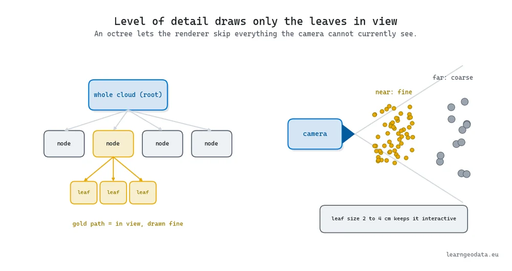
You index the cloud spatially so the renderer only touches points near the camera, and you build levels of detail so far regions draw coarse. Game engines have done this for decades, and the fix is always the data layout, not the hardware. Our guide to point cloud level of detail with an octree covers that structure step by step.
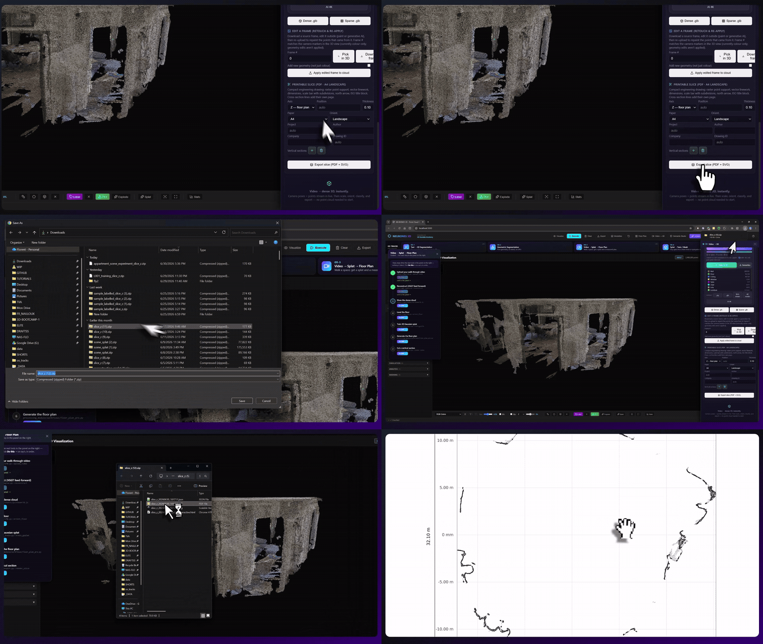
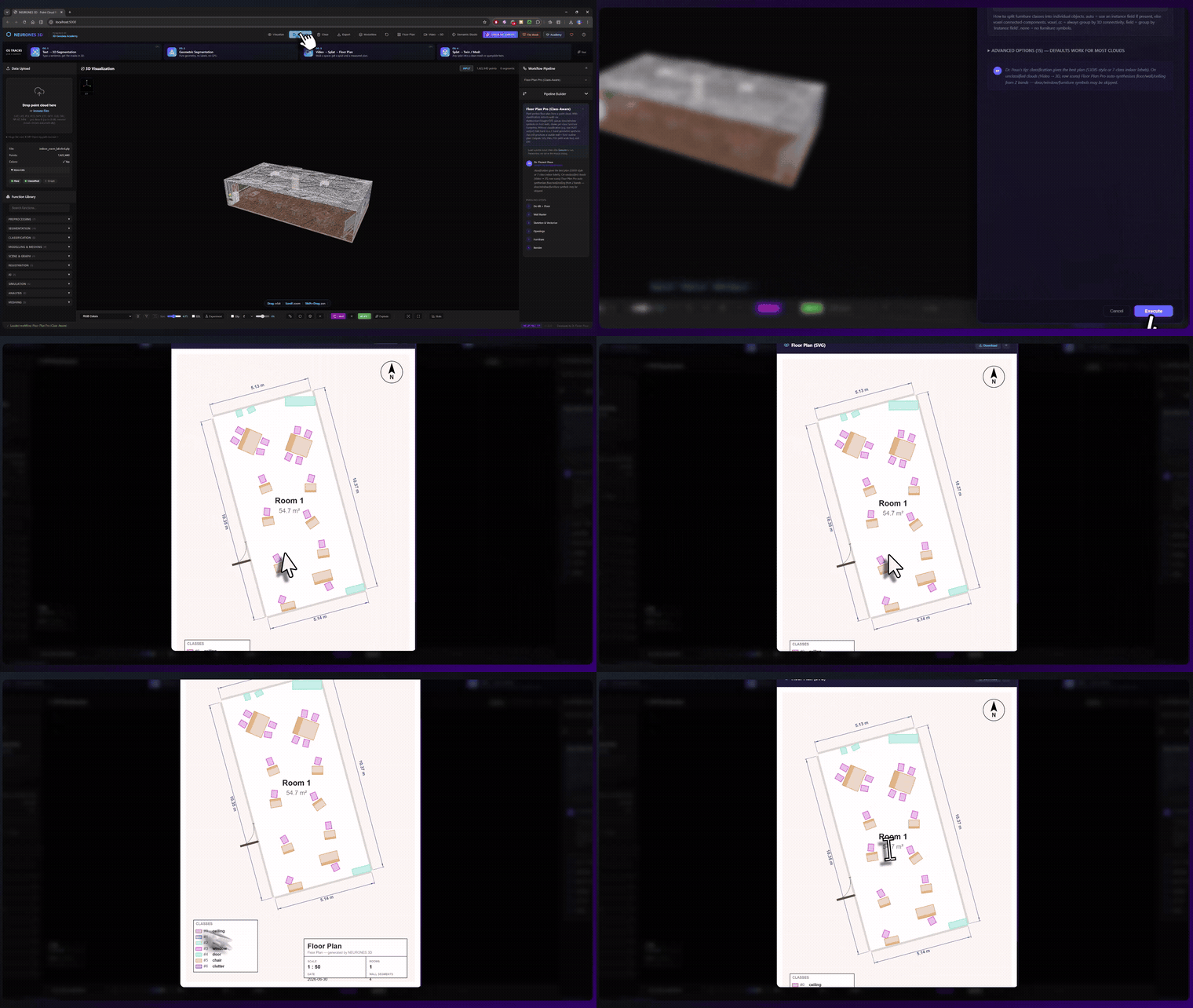
Sometimes you do not want to write a viewer at all, you just want to send a client a link. Potree streams enormous clouds into a browser with no install, and CloudCompare handles inspection and measurement on the desktop without a line of code. When you need cinematic output, Blender takes point data too and scripts in Python, so you can batch-render a hundred scans overnight with identical lighting.
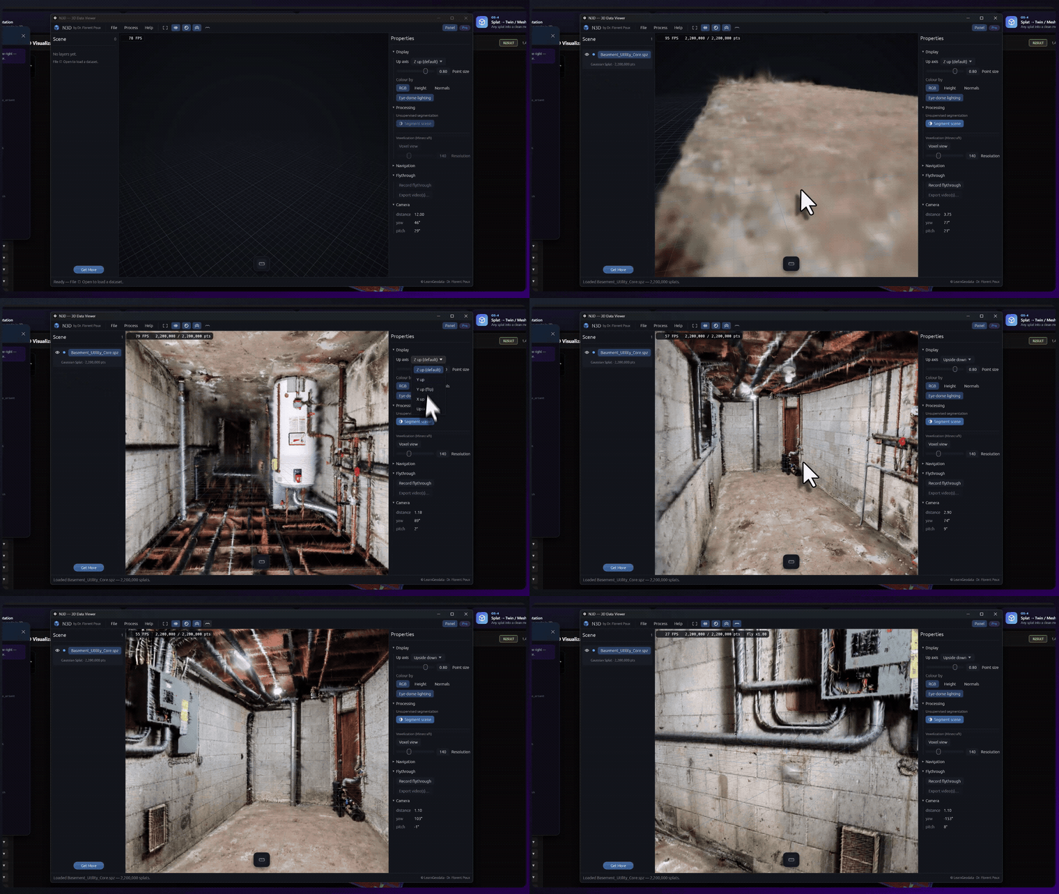
🪐 System Thinking Note: Level of detail transfers far beyond point clouds. An octree with a leaf size around 2 to 4 cm keeps tens of millions of points interactive on aging hardware, for the same reason web maps load tiles and video streams switch resolution: never pay to render detail the viewer cannot currently see. Learn it here and you’ll spot it everywhere data outgrows the screen.
Common Point Cloud To Mesh Pitfalls
Before you go build, here are the failures that eat your hours fastest, in the order they usually bite.
First, skipping normal orientation, the number one cause of inside-out meshes and a one-line fix you keep forgetting. Second, cranking Poisson depth to 12 on a whim and running out of memory, when depth 9 would have shown you the problem was upstream anyway. Third, forgetting to trim by density and shipping a mesh full of bubbles.
Fourth, comparing two scans without reporting the registration residual, so nobody knows which changes are real. And fifth, blaming your GPU for a slow viewer when the true fix is spatially indexing the data.
Notice the pattern? Almost none of these live in the reconstruction step everyone stares at. The weak link is usually one step earlier, in capture, normals, or registration.
🌱 Growing Note: Once your pipeline runs clean, break it on purpose. Add 5 percent noise, drop the Poisson depth to 6, skip the orientation call, and watch each stage fail on its own. The parameter intuition you build doing that is the thing no article can hand you, and it is exactly what carries over when you start feeding these surfaces into a 3D deep learning model.
Where This Fits In The Wider 3D Spatial AI Workflow
Point cloud meshing sits at the delivery end of a longer 3D spatial AI arc. If you want the raw material that feeds it, the companion guide on LiDAR and point cloud processing in Python covers ingesting and cleaning the clouds you mesh here, and the guide on open-vocabulary 3D segmentation covers labeling what those surfaces mean before you ship them. For the whole picture, the complete guide to 3D spatial AI with Python maps every stage in one place.
When you are ready to build a full system instead of a folder of scripts, the 3D AI Program takes each of these pieces from a working snippet to a production pipeline with feedback on your own data.
Your First Point Cloud To Mesh This Week
I used to think the answer to a bad mesh was always more cleanup and more parameters. It usually is not. Nine times out of ten the fix lives upstream, in a sensor choice or a skipped normal orientation, and staring at the reconstruction step just treats a symptom.
So try the smallest complete loop you can. Generate a synthetic room in a dozen lines of NumPy, or grab a scan you already own, and push it through the four Open3D calls above until a watertight surface shows up tonight.
Then go deeper deliberately. The free mission is a soft place to get that first system guided end to end, and the 3D AI Program is where you build the whole capture-to-render pipeline as one system. So which link in your own chain is the weakest one right now, the capture, the surface, or the view?
Frequently Asked Questions
Why Do My Poisson Meshes Have Weird Blobs Around The Edges?
Poisson always returns a closed surface, so in unscanned regions it invents geometry to seal the shape, and that shows up as balloons near the boundaries. The fix is to use the per-vertex density values the function returns and delete the lowest-density vertices, starting with the bottom 3 to 4 percent. The 3D AI Program walks this trimming step on messy production scans.
How Many Points Do I Need For A Clean Mesh?
There is no fixed count. What matters is even coverage of every surface you care about and enough overlap that no wall is a handful of stray dots. A dense, uniform capture meshes cleanly at modest sizes while a huge but patchy cloud still tears, which is why you plan capture density around the surfaces that matter, as the Open3D reconstruction docs show with their example datasets.
When Should I Pick Poisson Over Marching Cubes?
Reach for Poisson when you want a smooth, watertight surface from oriented points, which covers scanned buildings and objects. Reach for Marching Cubes when your data already lives on a grid or a volume, like a medical scan or a signed-distance field, a lineage that traces back to Lorensen and Cline’s 1987 paper. If your Poisson result looks bubbly, the problem is usually holes in the cloud, not the algorithm.
Do I Need A Powerful GPU To View Large Point Clouds?
No. The bottleneck for huge clouds is almost never raw GPU power, it is whether the data is spatially indexed so the viewer only loads what the camera can see. Browser tools like Potree stream billions of points out-of-core on ordinary hardware because they never hold the whole cloud in memory at once.
Can I Learn This Whole Workflow For Free?
Yes, and you should start there. Open3D and NumPy cover the loading, normals, and reconstruction, while CloudCompare handles inspection and measurement with no code, so a full capture-to-render pipeline costs nothing but your time.

