Open the maps app on your phone and zoom all the way out. You see a whole continent drawn as a handful of soft, blurry tiles. Now pinch into your own street, and the app quietly swaps those blurry tiles for sharp ones, but only for the little rectangle on your screen. It never downloads the planet at street resolution, because that would be terabytes and your phone would melt. That pyramid of pre-cut tiles, coarse at the top and fine at the bottom, with only the visible ones ever loading, is the cleanest way I know to understand point cloud level of detail. An octree is that same pyramid, in 3D, for a billion measured points.
What you’ll learn in this article:
- A precise mental model of the octree as a point cloud level of detail structure, not just a box for spatial search
- The four mechanics that make real-time point cloud rendering possible: level of detail selection, frustum culling, sparse voxel octrees, and out-of-core streaming
- When each one earns its keep, and when reaching for it is over-engineering
- A from-scratch Python demo that builds an octree and watches a far camera and a near camera spend the same budget completely differently
Estimated reading time: 14 minutes
Why a billion-point cloud needs level of detail
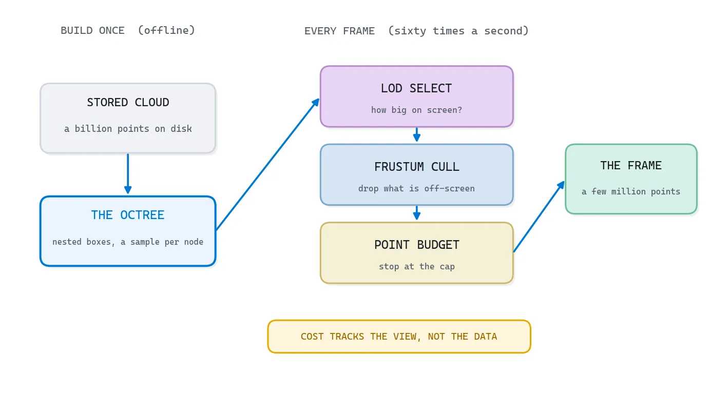
Let me set the constraint honestly, because the numbers are what make this fun. Say you have a billion points sitting on disk, around 30 GB of them. Your graphics card can comfortably draw a few million points per frame, nowhere near a billion. And your RAM might not even hold the whole file. Yet you still want to pan, orbit, and zoom without a single stutter.
So three separate walls stand in your way at once. The screen has only a few million pixels, so it cannot usefully show more than a few million points. The card cannot draw a billion per frame. And the machine cannot fit the cloud in memory. Each wall wants its own answer, and the elegant part is that one data structure sets up all three.
You already feel the move from the maps app. You do not fight the size of the world, you pre-cut it into tiles at every zoom level, so at any instant you grab exactly the slice the current view needs and ignore the rest.
The job is never to draw everything. It is to draw the least you can get away with and still be believed.
So what structure lets you ask “hand me the few million points that best show what the camera sees right now” and answer in a millisecond? That is the octree, and it is where we start.
🦚 Florent’s Note: Quick hello before we go deeper. It’s Florent. This piece sits a layer below my usual capture-and-extract tutorials, down in the plumbing that makes massive clouds feel weightless. If you have ever watched one viewer choke on a 2 GB file while another flies through 200 GB, the whole difference is in here. The demo at the end is CPU-only, no graphics card needed, so you can read every number it prints before you decide to trust it. Read it once top to bottom, then come back and run it.
The octree behind point cloud level of detail
A lot of introductions meet the octree as a spatial index, a way to ask what sits near a given spot. That is true, and it badly undersells the structure. The reason the octree is the backbone of point cloud level of detail is that every node also holds a usable little picture of the whole region beneath it. Think of a map tile at zoom level three: it is not nothing, it is a real, coarse view of a big area.
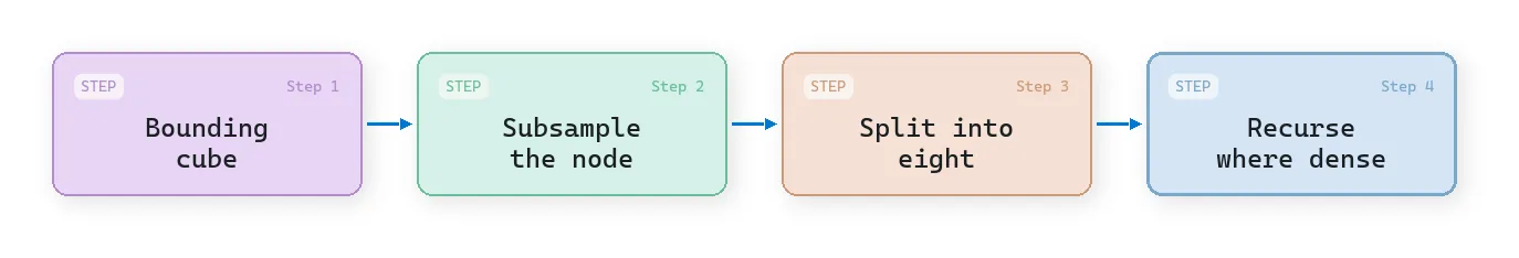
Here is the construction, and it is worth building in your head. Take the cube that bounds your entire cloud, and store a thinned subsample inside it, a few thousand points spread evenly. That root sample is a coarse portrait of the full dataset, your zoomed-all-the-way-out tile. Then split the cube into eight, split each of those into eight again, and at every node store another subsample of just that node’s points. The deeper you go, the smaller the box and the finer the detail.
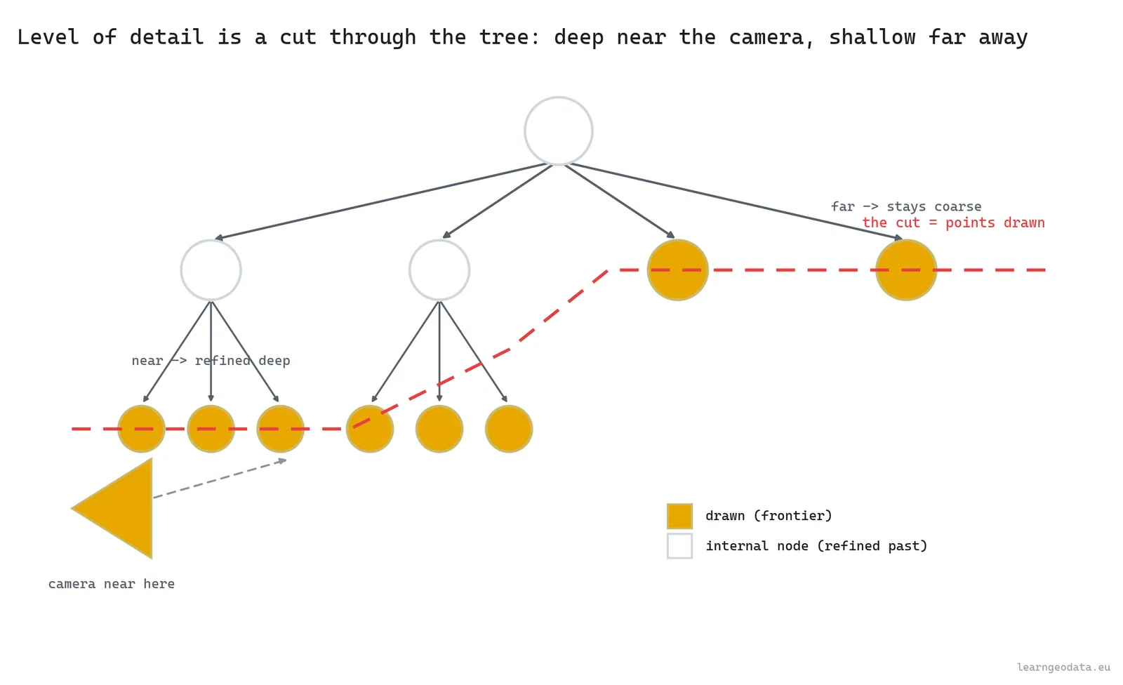
So a node is more than the points in this box. Actually, let me put it more precisely: a node is a fair sample of this box, at the resolution that matters for a box this size. That one design choice is what turns a storage tree into a rendering tree. When you draw, you walk down from the root and stop at the level that is detailed enough for the view, then draw that node’s sample. Stop high for far regions, descend deep for the part under your nose. The union of those stopping points is a clean cut through the tree, and it is a faithful picture at a fraction of the cost.
You can watch the structure form. The boxes appear level by level, and they only ever subdivide where points actually land, so empty air stays coarse and free.
🪐 System Thinking Note: What makes the pyramid honest is that the samples are nested and additive, not redundant. A parent’s sample plus its children’s samples together look like a denser version of the same region, because each level adds points the levels above lacked. That is the exact idea behind a mip-map in texturing, where each smaller image is a prefiltered version of the bigger one, and behind the slippy-map tile pyramid your browser fetches every time you pan. Build the hierarchy so coarse is always a fair summary of fine, and level of detail stops being a hack and becomes a property of the data.
The tree can hand you any resolution on demand. So how does a single frame decide which resolution each region actually deserves?
Point cloud level of detail: spend resolution where the zoom can use it
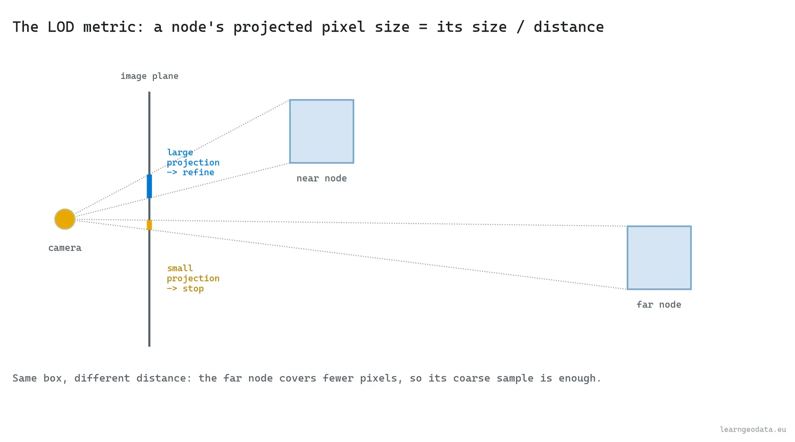
Here is the rule, and it is the same one the maps app applies a thousand times a second. A region far from the camera covers very few pixels, so drawing its full density is wasted, because a pile of those points lands on the same pixel. A region right in front of you covers many pixels, and it deserves every point you can give it. So you need one number: how much screen a node would take up.
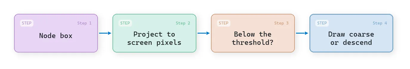
The standard number is the node’s projected size. You take the bounding-box diagonal in meters, divide by the distance to the camera, and scale by the focal length in pixels.
def projected_px(node, cam):
    """Screen-space size (pixels) of a node's bounding box, the LOD metric."""
    center = 0.5 * (node["min"] + node["max"])
    diag = np.linalg.norm(node["max"] - node["min"])
    dist = max(np.linalg.norm(center - cam["eye"]), cam["near"])
    return diag / dist * cam["focal_px"]
Is that projected size below a threshold, say a hundred pixels? Then the node’s coarse sample already matches what the screen can show, so you stop. Bigger than the threshold, and you descend to let the children refine it. Far node, large distance in the denominator, small projected size, draw it coarse. Near node, small distance, large projected size, descend and refine. The drawn cloud ends up dense where you are looking and a believable blur everywhere else.
This is where the point budget comes in. You set a cap, say two million points per frame, and you spend it on the nodes that matter most to the view: closest, largest on screen, coarsest detail still missing. Turn the budget up and the scene looks richer but the frame rate sags. Turn it down and you hold sixty frames a second at the price of some far-away crispness. So it is a single dial between fidelity and smoothness, and the right setting depends on the scene and the hardware.
Watch the level of detail move with the camera. The cloud thins to a coarse overview far away, then fills back in to full resolution as you dolly in, the same swap a map makes when you zoom into your street.
🦥 Geeky Note: Two numbers run this, and people set one while ignoring the other. The pixel threshold is taste, how sharp you want the foreground, and a tight threshold blows the budget fast on a busy view. The point budget is the hard ceiling that protects your frame rate. There is a third number hiding in the build: the points kept per node, the node capacity, where I use 2500. Too small and the coarse levels look threadbare when you zoom out. Too large and each tile is expensive to draw and the level-of-detail steps feel chunky. Tune the threshold for the look you want up close, then set the budget to whatever holds your target frame rate on the weakest machine you support.
Drawing the right detail still wastes effort if half of it sits behind you. So what is the cheapest thing we can refuse to draw at all?
Frustum culling for real-time point cloud rendering
The camera sees a shape like a pyramid with its tip sliced off, the view frustum, bounded by a near plane, a far plane, and four sides for the screen edges. Anything outside that shape simply cannot land in the frame. So the cheapest optimization there is tests each node’s box against the frustum and skips the whole node, plus its entire subtree, when it falls outside.

The payoff is enormous, because culling is hierarchical. If a node high in the tree falls fully outside the view, you discard millions of points with one box test and never touch its children. You are not deciding detail there, you are deciding existence, and that decision costs six comparisons.
def aabb_in_frustum(node, planes):
    """True if the node's box is at least partly inside the frustum (positive-vertex test)."""
    bmin, bmax = node["min"], node["max"]
    for a, b, c, d in planes:
        px = bmax[0] if a >= 0 else bmin[0]
        py = bmax[1] if b >= 0 else bmin[1]
        pz = bmax[2] if c >= 0 else bmin[2]
        if a * px + b * py + c * pz + d < 0:      # most-positive corner still outside
            return False
    return True
The test picks, for each plane, the single box corner farthest along that plane’s normal. If even that best-case corner is outside, the whole box is outside, and you cull. It is conservative, so it never hides something it should show, and it is six cheap comparisons for a whole subtree. That asymmetry, a tiny cost to throw away millions of points, is exactly why culling is the first lever you reach for. Watch it sweep: as the view turns, whole cells fall out of the draw set the instant they leave the cone.
🌱 Growing Note: Frustum culling is the easy half of “do not draw what you cannot see.” The hard half is occlusion culling, not drawing the points hidden behind a closer wall, and it is genuinely tougher because a point cloud has no surfaces to block with. People approximate it with a coarse depth pass or a hierarchical z-buffer. If your frustum culling already works and you still draw too much in a dense indoor scene, occlusion is your next move, not a fancier level-of-detail metric. Start there.
We have treated the octree as samples of points the whole way. Sometimes the smarter play is to make the tree itself the geometry. When?
Sparse voxel octrees: when the octree becomes the geometry
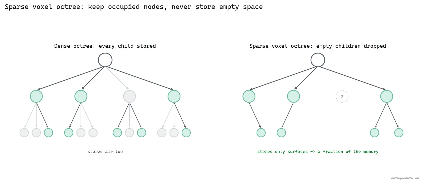
A sparse voxel octree, or SVO, flips the idea on its head. Instead of storing points and subsampling them, you store occupancy: each leaf is a voxel that is either full or empty, and the tree keeps only the nodes that contain something. The word sparse is the entire point. Empty space costs nothing, because empty children just do not exist in the tree.
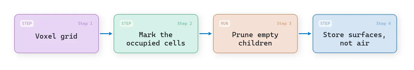
That buys two things. Memory, because a scene that is mostly air, and a lot of scenes are, stores only its surfaces. And fast ray traversal, because you can march a ray down the octree skipping big empty blocks in single jumps, which is how plenty of voxel ray tracing and volumetric rendering actually work. The reference here is Efficient Sparse Voxel Octrees by Laine and Karras at NVIDIA, who made this practical on a GPU.
So when do you pick an SVO over a point octree? When you care about solid-space queries, ray casting, or a fixed-resolution volumetric model more than about the original measured points. A point octree keeps every point and is perfect for fidelity and inspection. An SVO discretizes to a grid and is perfect for “is this cell occupied, and what surface does a ray hit first.” Different jobs, different tools.
🦚 Florent’s Note: Let me be honest about a mistake I have watched teams make, because I nearly made it once myself. They voxelize a beautiful survey-grade cloud into an SVO because it sounds modern, and they quietly throw away the very precision the client paid for. The grid resolution becomes the new accuracy ceiling, full stop, and you cannot get it back. Voxelize when you genuinely need the query speed or the ray traversal, never because it is the fashionable structure. If the deliverable is measurements, keep the points.
Point octrees, voxel octrees: both still assume the data fits somewhere you can reach it. What happens the day it does not?
Out-of-core point cloud rendering: streaming a cloud bigger than memory
Here is the wall that separates a toy viewer from a production one. Out-of-core means the dataset is bigger than your RAM, so it lives on disk, or across a network, and you stream pieces in and out as the view demands them. The octree is what makes this tractable, because the tree itself is a tiny index you can hold in memory while the bulk of the points stay on disk, one file per node.
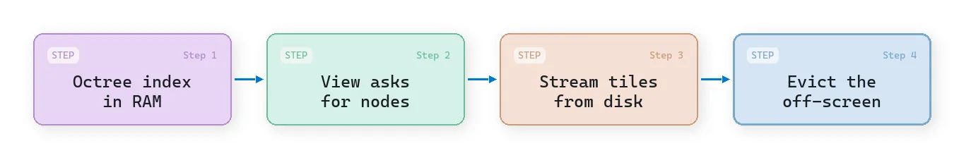
The loop is a paging system, the same one your operating system uses to pretend you have more memory than you do. Every frame, the level-of-detail pass decides which nodes it wants. The ones already in memory get drawn. The ones that are not get queued to load, asynchronously, so the render thread never blocks waiting on a disk. As the camera moves on, nodes that drift out of view get evicted to free up room. It is like a librarian reshelving the books behind you while you read the ones in front, so the desk never overflows.
The thing that decides whether this feels smooth or stuttery is prefetching. Load a node only the instant you need it, and the user watches it pop in late. Predict where the camera is heading and load the nodes it is about to want, and the data is already there when the eye arrives. This is the exact moment the maps-app analogy stops being an analogy and becomes the literal engineering: a streamable layout stores the octree so a viewer fetches one node with a single ranged read, even over plain HTTP from a static file.
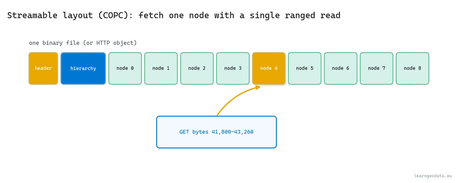
🦥 Geeky Note: The format matters more than people expect. A modern out-of-core layout, Potree‘s own format or the cloud-optimized point cloud (COPC, built on LAZ), bakes the octree into the file so a viewer fetches one node with a single byte-range request. That is why you can stream a 100 GB cloud from a static web server with no database behind it. The hierarchy is the index, the ranged read is the query, and the whole thing works because the tree was written in at conversion time. You can read and convert these with laspy and PDAL.
Four mechanics, one tree. So how do you choose which ones a given job actually needs?
When to reach for each point cloud level of detail trick
Let me make this practical, because the mechanics only help if you know when to spend them. Here is the short decision tree I carry in my head.
- A cloud that fits comfortably in memory, a few million points, a single room: you barely need any of this. Load it, draw it, maybe a simple grid subsample for when you zoom out.
- A cloud that is big but fits on the machine, tens to hundreds of millions of points: build the octree and use level of detail and frustum culling, but keep it all in RAM. This is the sweet spot for a desktop viewer, and where a lot of survey work lives.
- A cloud bigger than memory, or one you are serving to many users over the web: out-of-core is not optional. You build the octree on disk in a streamable format and accept the extra complexity of paging and prefetch.
- A problem about occupancy or ray traversal rather than fidelity: that is when the sparse voxel octree earns its place instead of the point octree.
🦚 Florent’s Note: Reaching for a full out-of-core pipeline on a small cloud is over-engineering, and I have watched people burn a week building streaming infrastructure for a dataset that fit in a laptop’s RAM twice over. So match the machinery to the wall you are actually hitting. If nothing is bigger than memory, do not pay for the disk paging you do not need. The cleverness is in spending exactly enough.
Enough theory. Let me show you the whole idea in code you can run tonight.
A runnable point cloud level of detail demo in Python
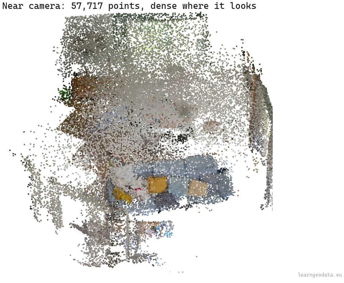
We will build an octree from scratch, give it the screen-space metric and the frustum test, and traverse it to a point budget from two different cameras. The payoff is the contrast: a far camera that draws the whole scene coarsely, and a near camera that spends the identical budget on fine foreground detail while culling everything off to the sides.
It runs CPU-only. In development mode it synthesizes a spread-out scene, a ground plane and a grid of box buildings, so the culling and the level of detail are easy to see. Point it at a real LAZ tile and the same traversal runs unchanged. One environment covers all of it:
conda create -n spatial_ai python=3.11 -y
conda activate spatial_ai
pip install numpy matplotlib laspy
There are no heavy dependencies on purpose. The octree, the camera math, and the culling are all NumPy, because the entire point of reading this is to see the mechanics with nothing hidden behind a library. To keep it honest, I run every step twice: on the synthetic scene, and on a real room scan of 2.18 million colored points. The mechanic first, then the same mechanic holding up on real data.
The traversal is where it all comes together, so read this part closely. We walk the tree best-first, always expanding the node that is largest on screen, culling anything outside the frustum, and refining a node into its children only while it is both big enough and within budget. When the budget runs dry, we stop and draw what we have. The whole policy lives in a single boolean:
refine = node["children"] and size >= lod_px and points + len(node["sample"]) < budgetRead those three conditions, because together they are the entire behavior. A node becomes its children only if it has children, and it projects bigger than the pixel threshold, and drawing those children will not bust the budget. Fail any one and the node draws at its own coarse sample instead. So that one line is level of detail, budgeting, and graceful degradation, all at once.
Now point one camera high and far back so it sees everything, and another down among the buildings looking across. Same tree, same budget, completely different spend.
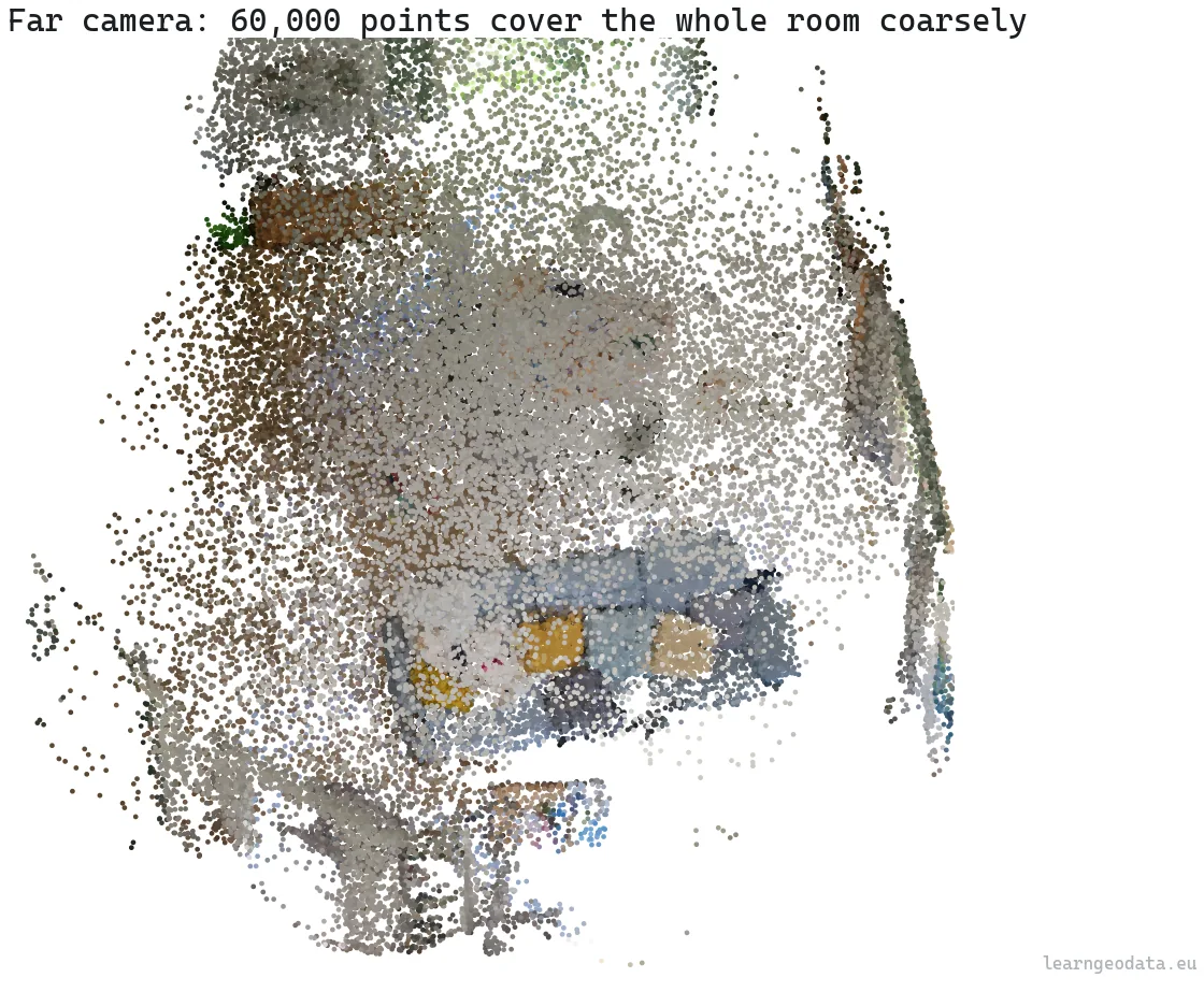
On my run, the far camera drew about sixty thousand points to cover the entire scene coarsely, and culled nothing, because nothing was off-screen. The near camera drew about the same sixty thousand points, but it poured them into the handful of surfaces in front of it, fine and dense, while culling whole nodes that fell to the sides. Same budget, same tree, and the detail followed the camera.
That is the whole idea in one comparison. The cloud never changed, only which slice of the tree best served the view, and the traversal found it in a fraction of a millisecond. So scale the cloud to a billion points and the tree just grows a few levels deeper, while the per-frame work barely moves, because you still only ever touch the cut.
The same octree that speeds up point cloud processing
Here is the part that surprised me the first time it clicked. The octree is more than a rendering trick. The same tree-over-space idea is what makes processing a point cloud fast, because almost every operation you run is a spatial query underneath. Estimating normals means finding each point’s nearest neighbors and fitting a plane. Building a segmentation graph, computing local descriptors, filtering the ground, detecting change between two scans: every one of them asks “what is near this point” or “what sits inside this region,” millions of times over.
Do that by brute force and you compare every point against every other point. Do it through a tree and you skip almost all of those comparisons. So I measured the gap on a labelled indoor scan of 1.42 million points, the index against brute force. The numbers are not subtle.
| Operation | Scale | Brute force | With the index | Speedup |
|---|---|---|---|---|
| Build the index (cKDTree) | 1.42M points | – | 417 ms | – |
| 16-NN, 2,000 queries | 300k points | 5,071 ms | 4.1 ms | 1,224x |
| Radius search (r = 0.15 m), 2,000 queries | 300k points | 3,246 ms | 26 ms | 126x |
| Voxel downsample (5 cm) | 1.42M points | – | 2,090 ms | 17.5x fewer points |
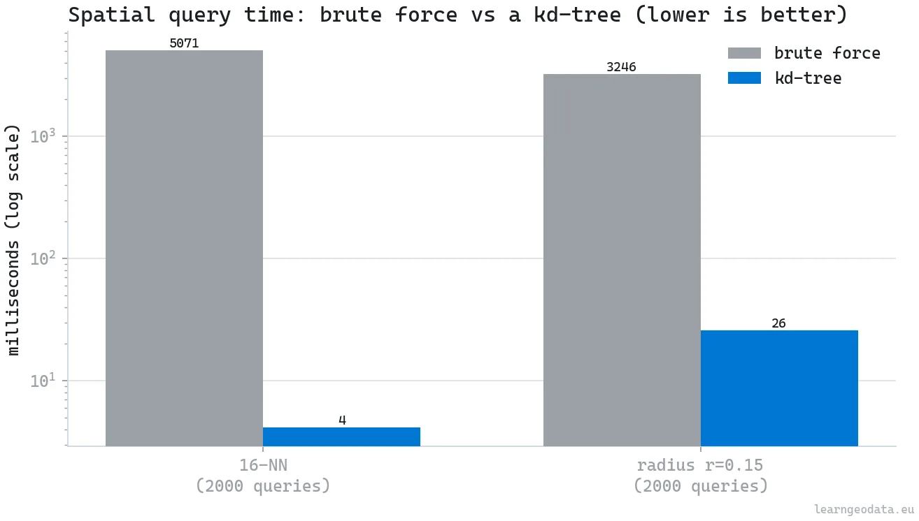
Read the second row again. A 16-nearest-neighbor query that takes five seconds by brute force takes four milliseconds through the tree, on the same data, for the same exact answer. That is not a tweak. It is the difference between a pipeline that runs and one that does not.
The honest caveat is the build cost. The tree took 417 milliseconds to construct on those 1.42 million points, and it holds memory while it lives. For a single lookup, brute force is fine and the tree is a waste. But the tree wins the instant you query it more than a handful of times, which processing always does, since normals alone are one query per point, millions of them. Build once, query a million times, and the 417 milliseconds vanishes into the noise. That amortization is the same logic as building the rendering octree once and drawing from it forever.
Where point cloud level of detail breaks, and how to ship anyway
Let me be blunt about the trade-offs, because none of this is free, and trusting it blindly will burn you. The first visible cost is popping. When you move and a region crosses a level-of-detail threshold, its detail jumps in one step and your eye catches it. Good viewers hide this by blending between levels or loading the next level early, but a naive implementation visibly snaps. The second cost is sample quality. Random subsampling, like in the demo, makes the coarse levels look noisy, and doing it well with a Poisson-disk style sample takes real care at build time. And third, the tree is not free to make. Converting a big cloud into a streamable octree can take minutes to hours and a chunk of disk, and that cost lands before anyone sees a single frame.
None of these kill the approach. They are the bill, and you should know it before you promise someone sixty frames a second on their data.
🌱 Growing Note: Here is the one upgrade I would make first in production: do not ship a fixed point budget. The budget that holds sixty frames a second on your workstation will stutter on a five-year-old laptop and waste a high-end one. Make it adaptive, measure the actual frame time, nudge the budget down when frames run long, and up when there is headroom. A fixed budget is a promise you can only keep on the exact machine you tuned it on. An adaptive one is a promise you can keep everywhere.
Step back and the through-line is simple. Every technique here is a way of spending a scarce resource only where it changes what someone perceives: level of detail rations pixels, frustum culling rations the card, out-of-core rations memory, the budget rations the frame. Once you see rendering as rationing against perception, you stop asking “how do I draw it all” and start asking “what is the least I can draw and still be believed.” That second question scales to a billion points. The first one never will.
Build your first level-of-detail point cloud this week
Reading about this is not what makes it click. Doing it once is.
So do one concrete thing. Take the demo, point it at a real LAZ tile instead of the synthetic scene, and print the stats from a few camera positions. Watch the drawn-point count hover near the budget while the cloud behind it could be any size at all.
Then feel the disconnect between the data’s size and the frame’s cost, because that disconnect is the whole point of everything above. Once you have seen a million-point cloud and a billion-point cloud cost almost the same per frame, you understand why this structure won.
If you want the structured path, from capture and registration through the data structures and the rendering that sits on top, I put the foundations into a free starting mission you can begin right now: start the free mission. And once you are hungry for the full stack, the academy’s course library goes from here to production. If you would rather see the semantics side first, here is a related walkthrough on open-vocabulary 3D semantics in Python.
So what is the first cloud you would point this at, and how big would you dare to make it before the frame rate even noticed?
Resources for point cloud level of detail and real-time rendering
- Potree, the open-source WebGL renderer that popularized out-of-core octree streaming for point clouds, by Markus Schütz and contributors.
- Potree: Rendering Large Point Clouds in Web Browsers, the foundational thesis on the octree streaming approach, straight from the source.
- Efficient Sparse Voxel Octrees, Laine and Karras, the reference for SVO ray traversal on the GPU.
- The COPC specification, the cloud-optimized point cloud format that bakes the octree into a LAZ file for ranged reads.
- Open3D, for point cloud I/O, octrees, and voxel grids in Python.
- laspy and PDAL, for reading LAS and LAZ and building conversion pipelines.
- The 3D Geodata Academy, where I teach this from capture to real-time rendering, with production code and the parameter intuition a single article cannot hand you.
I’m Florent Poux, Ph.D. I research and teach spatial AI, and I wrote 3D Data Science with Python (O’Reilly). I spend my days turning research into systems that ship, and my goal here is to give you the foundations the tools sit on top of.
Frequently asked questions about point cloud level of detail
What is level of detail in point cloud rendering?
Level of detail means drawing fewer points for regions that cover little of the screen and more for regions up close. An octree stores a subsample at each node, and the renderer descends only where a node projects larger than a pixel threshold, so you draw detail only where the viewer can use it. Libraries like Open3D expose octrees you can build this on.
How does an octree make point clouds render faster?
An octree splits space into nested cubes and stores a representative subsample at every node, so the renderer picks a coarse or fine level per region, culls whole subtrees that are off-screen, and stops at a point budget. The approach was popularized for the web by Potree, which streams clouds of hundreds of billions of points in a browser.
What is a sparse voxel octree, and when should I use one?
A sparse voxel octree stores occupancy instead of points: each leaf is a full or empty voxel, and empty children are not stored at all, so memory tracks surfaces rather than volume. It is ideal for ray traversal and solid-space queries rather than measurement fidelity, as detailed in Laine and Karras.
What does out-of-core rendering mean for point clouds?
It means the dataset is larger than memory, so it lives on disk and nodes stream in and out by view demand, with the octree as a small in-memory index. Streamable formats like COPC, readable with laspy and PDAL, let a viewer fetch one node with a single ranged read over HTTP.
Does the octree help with point cloud processing, or only rendering?
Both. The same tree accelerates spatial queries, so a 16-nearest-neighbor search that takes five seconds by brute force takes about four milliseconds through the tree, a roughly 1,224x speedup on a 1.42 million point scan. That is the lookup behind normals, descriptors, and segmentation, which you can learn end to end at the 3D Geodata Academy.

