

A multimodal foundation model is a pair of encoders trained together so that a picture and a phrase land at the same address in one shared vector space. Applied to 3D assets, you render each region of a scan, encode those frames with a frozen backbone, and add the measurements only your own survey holds.
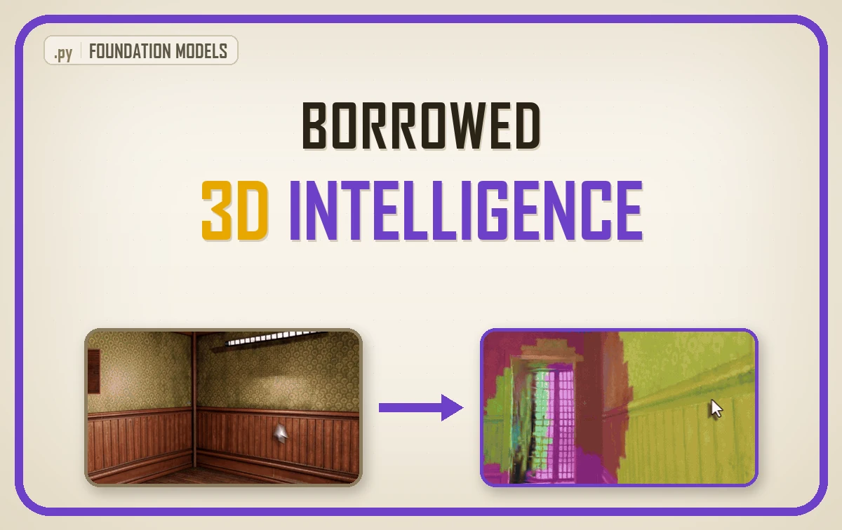
| What it is | A pretrained image and text model reused on 3D data, with no new backbone trained anywhere in the pipeline |
| What you build | One 1,295-dimensional region descriptor: CLIP 512, DINOv2 768, and fifteen numbers only your survey holds, plus a small head on top |
| Libraries | open_clip, PyTorch, Open3D, NumPy, scikit-learn |
| Worked on | Two floors of one real indoor survey: 1,454 regions to train on, 1,603 held-out regions scored |
| Level | Intermediate to expert. Assumes Python, PyTorch and basic point cloud handling. |
So what happens the first time you point a frozen backbone at a room it has never seen and ask it, in plain English, to find the windows?
The guide follows the order you would actually build this in, opening with what a foundation model gives you and closing with the geometric checks that catch its mistakes. Here is the path:
- What a Multimodal Foundation Model Is
- Why There Is No Foundation Model for Point Clouds
- Four Ways to Bridge Points Into a Pretrained Model
- How to Photograph a 3D Region So a Backbone Can Read It
- What to Freeze and What to Train
- The Geometry a Photograph Cannot Carry
- How to Search a 3D Scan With a Plain Sentence
- How to Evaluate Multimodal 3D Models Honestly
- Where Multimodal 3D Pipelines Go Wrong
- Five Multimodal 3D Mistakes and How to Fix Them
- Where to Go Next With Multimodal Foundation Models
- Run Your First Multimodal 3D Experiment This Week
- Frequently Asked Questions About Multimodal 3D Models
The implementation stopped being the hard part a while ago. Ask for a rendering loop, a pooling function, an evaluation harness, and back comes something that runs.
What no model will do for you is choose the evidence. It will not notice that a photograph carries no unit of length, so a coffee table and a helipad look identical to it.
That choice is the science, and it is the scarce ingredient in this field right now.
You arrived with a blunter version of the same question, though. You have an archive of scans, a GPU idle overnight, and no labelling budget anybody was ever going to sign off. Can you point one of these enormous pretrained models at your own 3D data and get something back that a client would pay for?
Short answer: yes, and the interesting part is which half of the work stays yours.
What Linnaeus Teaches 3D Naming
Carl Linnaeus published Species Plantarum in 1753 and gave every plant a two-word name. It sounds like bookkeeping. It was infrastructure.
A botanist in Uppsala could describe a specimen and a botanist in Nagasaki could recognize it, because both had agreed in advance on where a name lives. Two people who had never met could point at the same thing.
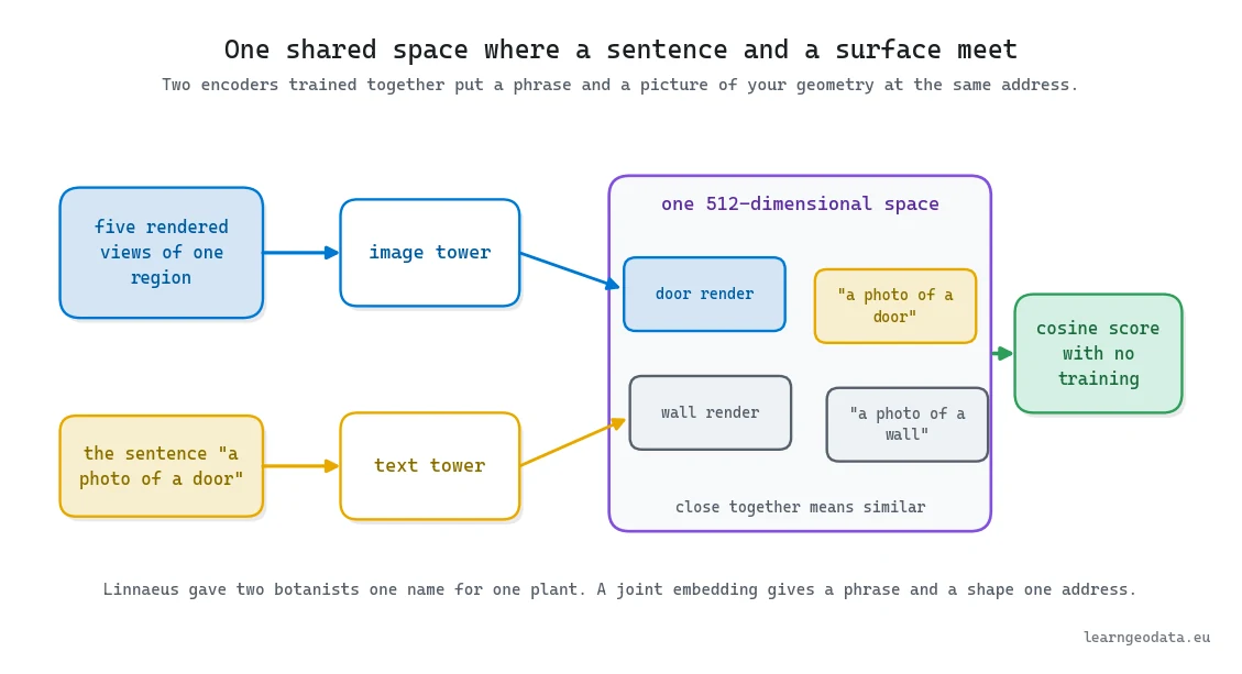
That agreement is what a multimodal foundation model hands you for free. A phrase and a picture get sent to the same address in one shared space, so a dot product between them means something. Your job is getting your geometry into that space.
What you will learn in this article
- What a multimodal foundation model is, and why the shared space is the product
- Why 3D and text pairs are scarce, and what that scarcity forces you to do instead
- Four ways to bridge irregular points into a pretrained backbone, with each trade-off priced
- What to freeze, what to train, and the label count that decides between them
- How to evaluate honestly, and the failure patterns to expect before you ship
What a Multimodal Foundation Model Is
A multimodal foundation model is two encoders trained against each other on a colossal pile of paired examples. One reads images, one reads text, and training pushes matching pairs together while shoving mismatched pairs apart, until a caption and its photograph become nearly the same vector.
CLIP is the canonical case, trained on hundreds of millions of image and caption pairs scraped from the open web. DINOv2 is the useful counterweight, trained with no language signal at all, learning structure by comparing views of the same image against each other.
So what do you actually download? Not a classifier. A function that turns a picture into a few hundred numbers, plus a promise that similar things land near each other. That promise is the asset.
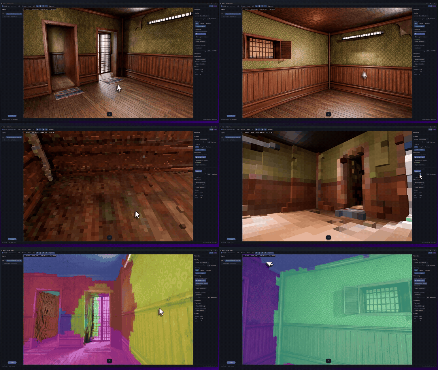
Which is why the multimodal half matters more than the foundation half. A single-modality model gives you a good descriptor. A multimodal one adds a door that English can walk through, and that door turns a segmentation pipeline into something a non-specialist can drive.
🦥 Geeky Note: Two frozen towers on one RTX 3090 pushed 263 views per second on the training split and 270 on the held-out one, peaking at 1,989 MB of VRAM at batch size 96. On that same held-out split the rasterizer feeding them managed 30 views per second, nine times slower, which tells you exactly where your optimization effort belongs.
Why There Is No Foundation Model for Point Clouds
Nobody ships a CLIP for point clouds because the paired data does not exist, and the arithmetic behind that is brutal rather than temporary.
Image and caption pairs number in the billions, harvested from a web that has been captioning photos for twenty years. Captioned 3D shapes number in the low millions, and a large share of those are synthetic objects sitting on white backgrounds. Pool every public benchmark of labelled indoor scans ever released and you reach a few thousand rooms. Your own asset classes, the ones a client pays for, exist in exactly one place.
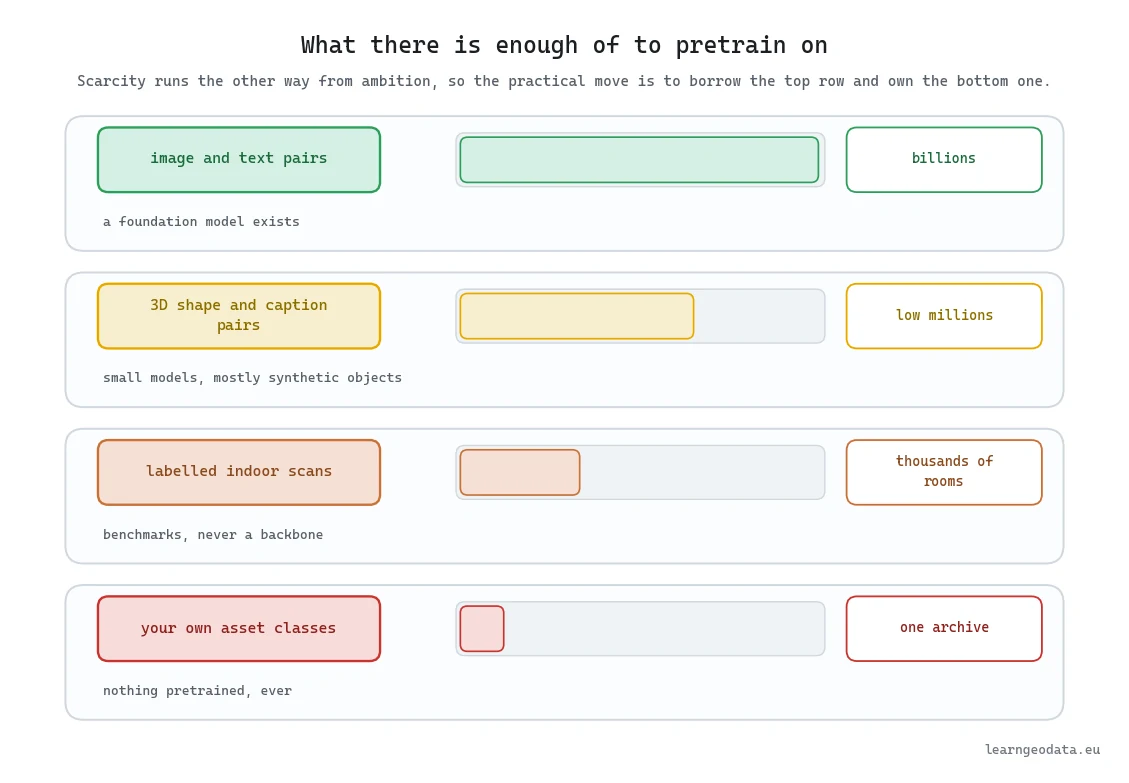
Read that gradient the right way and it stops being depressing. You are not competing with whoever trained the top row, because they cannot see your bottom row. Their weights improve every year at their own expense, and your archive improves only when you do the work.
The practical move is a division of labour. Borrow the vision already sitting inside the 2D models, engineer the crossing from unordered coordinates into a form those encoders accept, and keep the final stage for yourself.
Four Ways to Bridge Points Into a Pretrained Model
Four bridges carry irregular points into a pretrained model, and picking the wrong one costs you weeks: render and embed, a native 3D encoder, lifting 2D embeddings onto points, or geometry with no backbone at all.
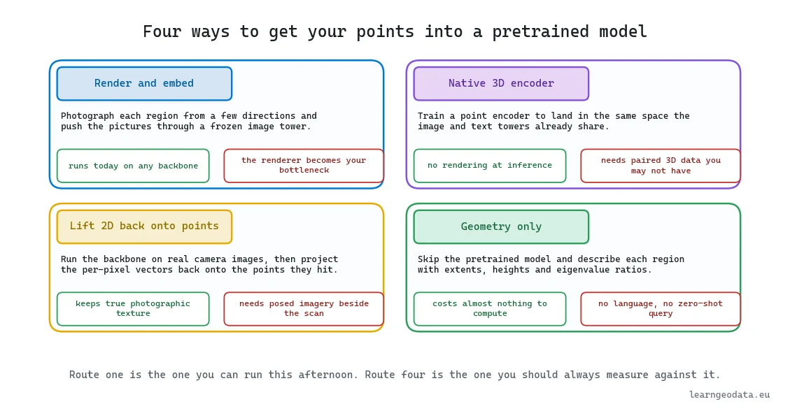
Render and embed is the one you can run this afternoon. Cut the scene into candidate regions, photograph each from a handful of directions, push those pictures through a frozen image tower. Nothing about the backbone changes, so it works with whatever checkpoint you downloaded this morning, and the price is a renderer that becomes your bottleneck in both compute and quality.
A native 3D encoder skips the camera entirely. You train a point encoder to land in the space the image and text towers already occupy, which is what Point-Bind and Point-LLM do and what PointLLM extends with a language model on top. Inference gets fast and clean, and training wants paired 3D data, which loops straight back to the scarcity problem.
Lifting 2D embeddings onto points inverts the first route. Rather than render synthetic views, you run the backbone on the real camera images your scanner already captured and project each pixel’s vector back onto the points it hit. Genuine photographic texture, at the price of posed imagery that plenty of archives simply do not have.
Geometry alone is the route people skip and the one you should always measure against. Extents in metres, height above the floor, eigenvalue ratios, colour statistics. No language, no zero-shot query, almost no compute.
Priced side by side, the four stop looking like a matter of taste.
| Bridge | What it needs from you | What it really costs | Pick it when |
|---|---|---|---|
| Render and embed | Candidate regions and an offscreen renderer | Throughput: the rasterizer managed 30 views per second against the encoder’s 263 | You want an answer this afternoon, on weights you did not pay for |
| Native 3D encoder | Paired 3D and text data | Training a point encoder into somebody else’s space, and the paired data to do it | You already hold paired 3D data, or the research question is the point |
| Lifting 2D embeddings | Posed camera images from the capture itself | Pose accuracy, and an archive that kept the imagery at all | Your scanner saved oriented photographs alongside the geometry |
| Geometry only | One covariance per region | Almost nothing, and you give up every text query | Always, as the baseline: 15 hand-written numbers reached 0.568 on the held-out floor |
The last row is the one people quietly skip. Build it first, because every claim you make about a backbone later is a claim about the distance between that backbone and those 15 numbers.

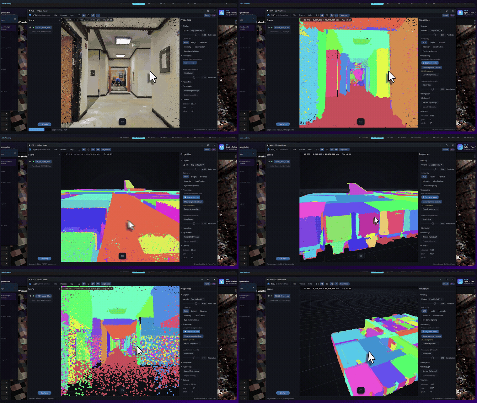
One decision sits upstream of all four. You need candidate regions first, because a foundation model classifies things and a point cloud is not a thing until you cut it into some. Get that cut wrong and no backbone recovers, so start at 3D point cloud segmentation and clustering in Python if region proposals are new to you.
🪐 System Thinking Note: Notice what you are really choosing between. A frozen backbone is a supplier relationship: fixed interface, a price of zero, a failure profile somebody else published. The moment you unfreeze it, you have taken delivery of its retraining schedule, its licence terms and its reproducibility for the life of the product. Treat it as a procurement decision, count the 238 million parameters you would be adopting, and the answer arrives fast.
How to Photograph a 3D Region So a Backbone Can Read It
The photograph decides your result far more than the backbone does, and the measured evidence is unambiguous. Keep a pale grey ring of neighbouring points around each region and a held-out floor comes back at 0.654 accuracy. Delete that ring, change nothing else, and the same head scores 0.639.
I want to be blunt about the version of this I used to repeat, because that version turned out to be wrong. The obvious design welds five cameras to the world axes and shoots every region on its own, with nothing else allowed into the frame. It scores badly. Fixing it meant changing two things at once, and for a long time I credited the wrong one. So every region on both floors was re-rendered under three view builds and scored by the same head at the same seed, which is the only way anybody finds out.
Derive the cameras from each region’s own surface and leave the ring in, which is the build this pipeline ships, and you get 0.654. Weld the cameras to the world axes and keep the ring, and you get 0.661. Keep the surface cameras and delete the ring, and you get 0.639. Retrain any of the three under eight head seeds and it wobbles by 0.003 to 0.005, which is the ruler you read all three against.
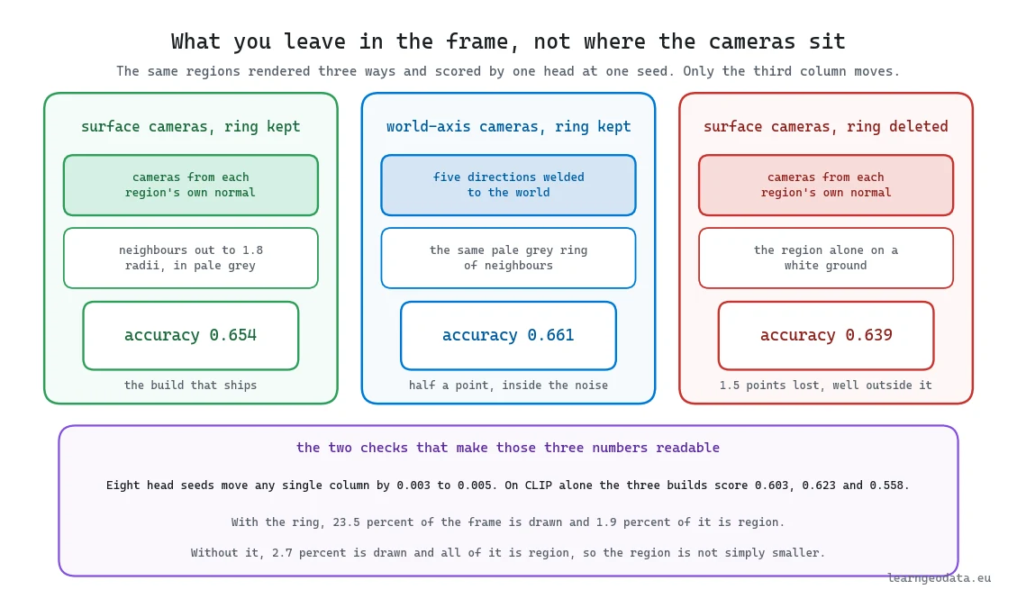
Read those three in order and the cameras drop out of the story. The world-axis build I had written off finishes half a point ahead of the careful one, about one standard deviation of seed noise, so this data cannot separate them. The ring is where the signal lives. Delete it and the full descriptor surrenders 1.5 points, while CLIP on its own surrenders 4.5, sliding from 0.603 to 0.558.
Before you believe an interesting explanation, kill the boring one. Perhaps the region simply renders smaller without its neighbours and the loss is really about resolution. A one-minute coverage script settles it. Ring in place, points cover 23.5 percent of the frame and only 1.9 percent of that frame is the region itself. Ring gone, coverage falls to 2.7 percent and the region owns all of it. Your region takes up slightly more of the picture once its neighbours leave, not less. What disappeared is everything standing around it.
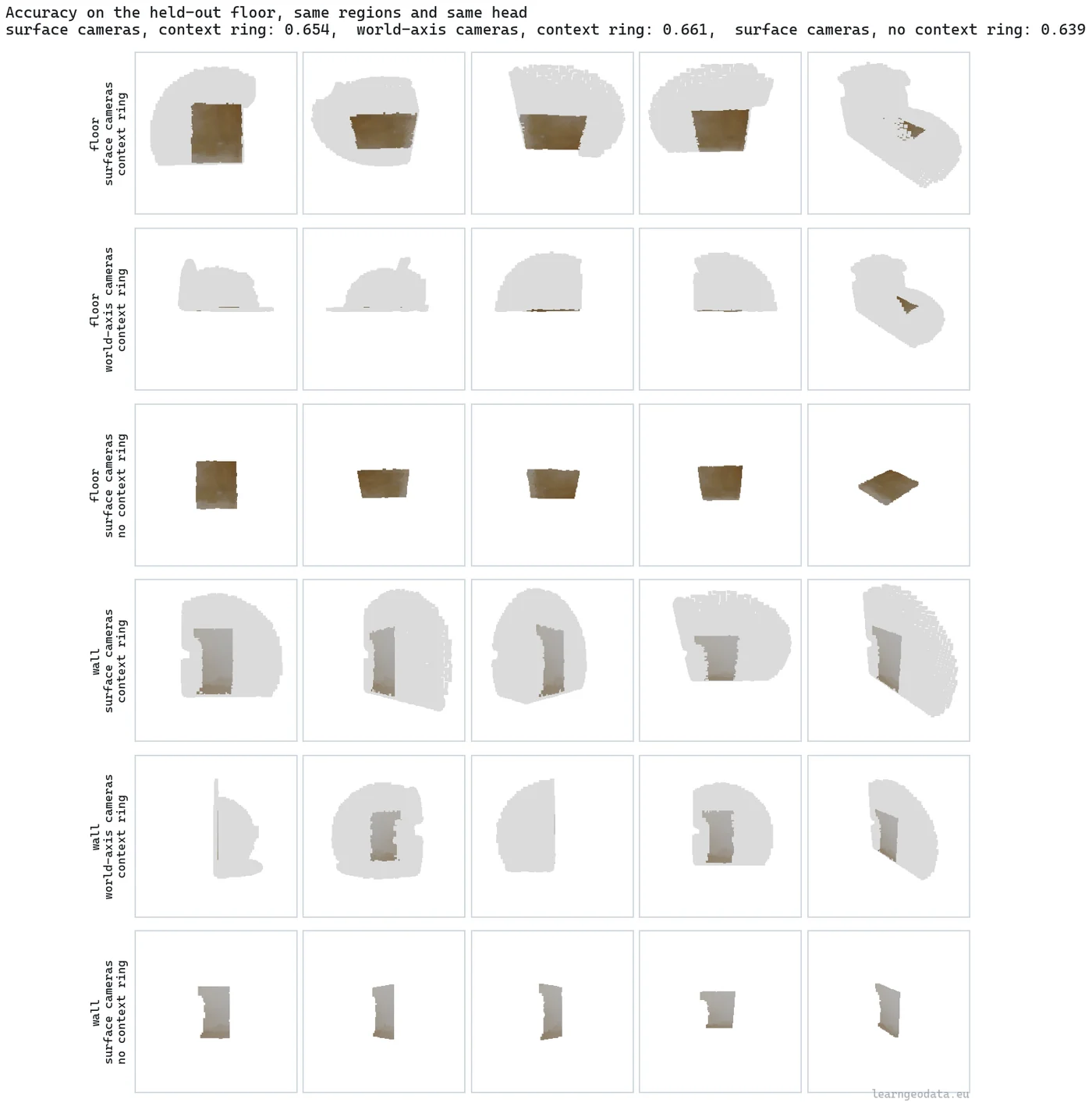
Keep the surface-relative cameras if you like them, and I do. The region’s mean normal becomes the primary view direction, flipped to look from the empty side, three further cameras tilt 48 degrees away from it inside the tangent plane, and one stays bolted to the world axes so gravity still reads somewhere. The reasoning holds up on paper and this dataset cannot detect any of it. Recentring each region and dividing by its own radius still earns its keep for a different reason, because it stops absolute scale being smuggled through the pixels and hands it to the geometric descriptors instead.
Here is the encoding pass once the renders exist. The uint8 frames go straight to the GPU with no image-library round trip, and pooling happens after the backbone.
import numpy as np
import open_clip
import torch

DEVICE = "cuda" if torch.cuda.is_available() else "cpu"
MEAN = torch.tensor([0.4815, 0.4578, 0.4082], device=DEVICE).view(1, 3, 1, 1)
STD = torch.tensor([0.2686, 0.2613, 0.2758], device=DEVICE).view(1, 3, 1, 1)

model, _, _ = open_clip.create_model_and_transforms(
    "ViT-B-32", pretrained="laion2b_s34b_b79k")
model = model.to(DEVICE).eval().requires_grad_(False)   # nothing here trains


@torch.no_grad()
def region_descriptors(views, batch=96):
    """views: (n_regions, n_views, 224, 224, 3) uint8 renders from one scan."""
    n_regions, n_views = views.shape[:2]
    flat = views.reshape(-1, *views.shape[2:])
    out = np.zeros((len(flat), model.visual.output_dim), np.float32)
    for start in range(0, len(flat), batch):
        chunk = torch.from_numpy(flat[start:start + batch]).to(DEVICE)
        chunk = chunk.permute(0, 3, 1, 2).float().div_(255)
        chunk = (chunk - MEAN) / STD
        out[start:start + batch] = model.encode_image(chunk).float().cpu().numpy()
    pooled = out.reshape(n_regions, n_views, -1).mean(1)     # order-independent
    norms = np.clip(np.linalg.norm(pooled, axis=1, keepdims=True), 1e-9, None)
    return pooled / norms
Two lines earn their keep. The mean over the view axis makes a descriptor independent of how many cameras survived, so a degenerate view can be dropped without rescaling anything. The division by the norm puts every region on the unit sphere the text tower already lives on, which is what makes the text search further down free. Check open_clip.list_pretrained() before hard-coding a checkpoint name, because the open_clip tags move between releases.
That mean deserved a measurement rather than a habit, so it got one. Max pooling scores 0.663 on the same head and split, mean and max concatenated 0.672 at double the width, and a parameter-free attention weighting each view by its cosine to the region’s own average lands at 0.657. The plain mean comes last of the four at 0.654, and it ships anyway, because the text search needs a mean-pooled unit vector living inside CLIP’s own space. If you never intend to type a sentence at your scan, take the 1.8 points.
🦚 Florent’s Note: I spent a long time telling people the camera rig rescued this pipeline, and the number I quoted for it does not reproduce. What does reproduce is duller and far more useful: the cameras are worth nothing, and the grey ring is worth 1.5 points on the full stack and 4.5 on CLIP alone. Think about why. Photograph a bare patch of wall, then a bare patch of door, and you have taken the same picture twice. Only the metre and a half of neighbourhood around each one tells them apart, so the question to put to your renderer is not where the cameras sit, it is what you are cropping out.
What to Freeze and What to Train
Your label count decides what you freeze and what you train, and with one labelled floor the answer is to freeze everything and train a small head on top of it.
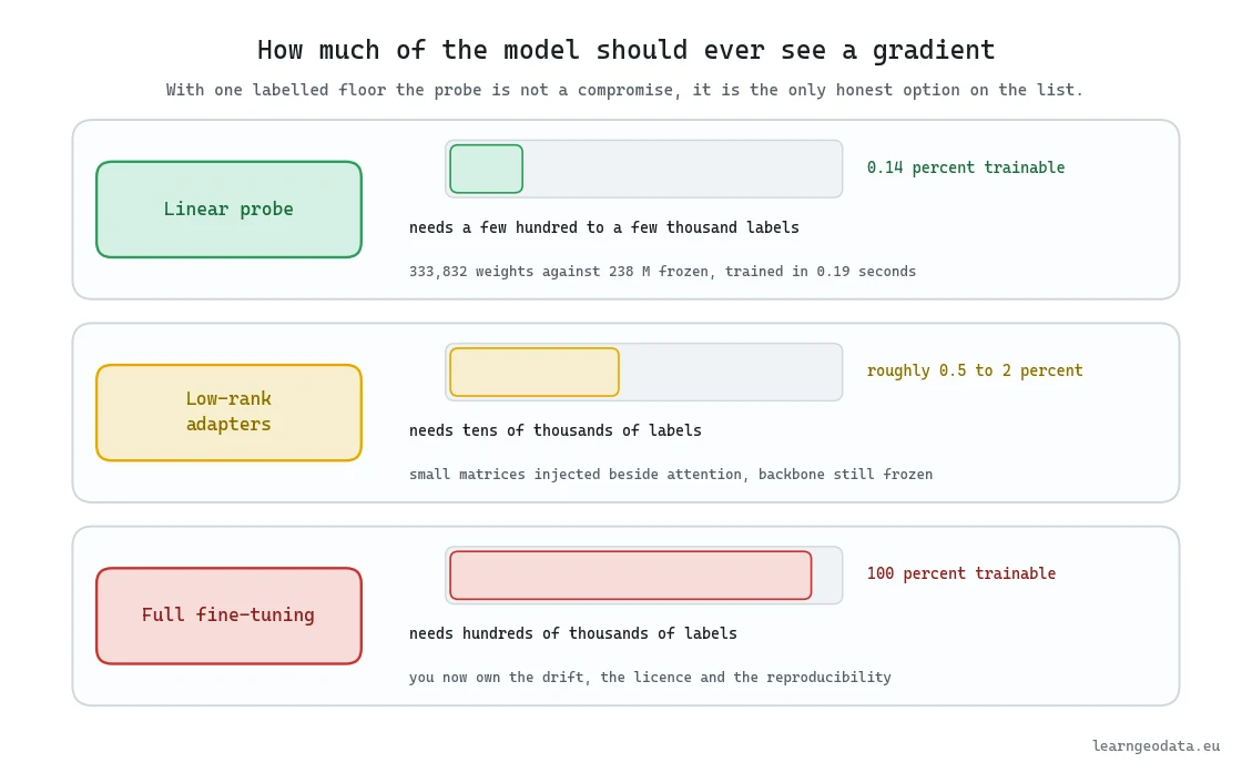
A probe trains that small head on frozen embeddings. On the pipeline behind this guide it held 333,832 parameters against 238 million frozen upstream, 0.14 percent of the total, and 140 full-batch epochs finished in 0.19 seconds. On 1,454 training examples whose renders had taken ten minutes to produce.
Low-rank adapters sit in the middle. Small matrices get injected beside the attention weights and trained while the backbone stays frozen, typically moving half a percent to two percent of the parameters. They repay you at tens of thousands of labels, once the frozen descriptors have visibly stopped improving.
Read the ladder by the only number that decides it, which is how many labels you actually hold.
| Labels you actually have | What you train | Share of parameters moved | What it costs you |
|---|---|---|---|
| Under a few thousand | A small head on frozen embeddings | 0.14 percent, 333,832 against 238 million | 0.19 seconds of fitting, and ten minutes of rendering before it |
| Tens of thousands | Low-rank adapters beside the attention weights | Roughly 0.5 to 2 percent | A retraining schedule and a licence you now own |
| Hundreds of thousands | Every weight in the backbone | 100 percent | A label budget one building never supplies |
Full fine-tuning puts a gradient through every weight, and the label count it wants is not something one building will ever supply. With a single labelled floor, the probe is not a compromise you settle for. It is the only defensible option on the list.
Notice where the time went in that first row. Fitting the head took 0.19 seconds and producing the pictures it learned from took ten minutes, which is a ratio of about three thousand to one. The rasterizer running at 30 views per second against an encoder that eats 263 is the same story from the other end. Optimize the renderer, cache the descriptors to disk, and treat the head as free, because on this ladder it is.
🌱 Growing Note: When your labels do grow past what a 333,832-parameter probe can absorb, the practical path is the Hugging Face PEFT documentation rather than a full unfreeze. Add adapters to the last few attention blocks only, keep the exact same evaluation harness, and measure the honest delta against the probe. If it comes in under two points, you just learned something useful for free.
The Geometry a Photograph Cannot Carry
Geometry is the evidence a photograph cannot carry. Pixels hold no unit of length, so a backbone trained on the open web cannot tell you whether the flat surface in front of it is a coffee table or a helipad, because nothing in its training ever put a ruler beside one.
Your scan has that ruler for free, and handing it over costs one covariance per region.
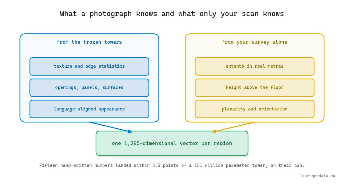
Fifteen numbers cover it: three bounding extents for absolute size, mean and minimum height for position in the building, the sorted eigenvalues of the point covariance for linearity, planarity and scatter, the mean normal for orientation, and three colour statistics for the material hints the renders wash out. Those 15 columns join CLIP’s 512 and DINOv2’s 768 to make the 1,295-dimensional descriptor.
Two of them repay a second look. Feed the point count through a base-ten logarithm first, since your regions will differ in size by a factor of a thousand and a raw count would swamp everything else in the standardized vector. Then add blue minus red as a crude daylight detector, because glazing photographs cool and dim while the plaster around it photographs warm.
🦥 Geeky Note: Standardize those 15 columns with the training split’s mean and standard deviation only, then apply the same constants to the test split. Skipping that two-line detail leaks the test distribution’s scale back into training, and it quietly inflates every number you are about to report.
How to Search a 3D Scan With a Plain Sentence
Searching a scan with a plain sentence costs one matrix multiply and no training at all, because CLIP’s two towers came out of a single run against one enormous pile of captioned photos, which puts your pooled region vector and a typed phrase on the same coordinate system.
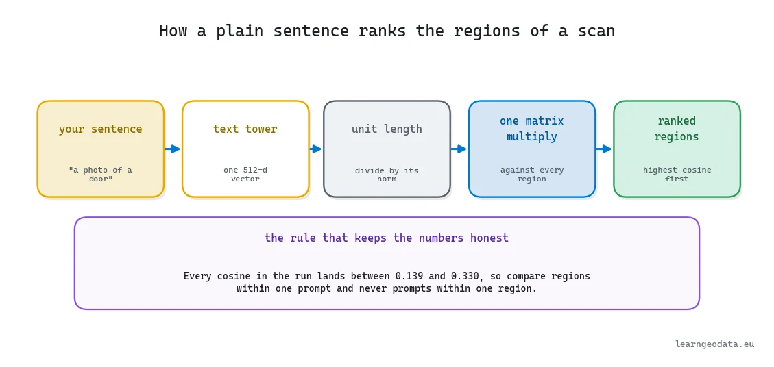
The implementation is short enough to read in one breath, which is why it is worth understanding rather than copying.
import numpy as np
import open_clip
import torch

tokenizer = open_clip.get_tokenizer("ViT-B-32")   # same tag as the image tower

PROMPTS = ["a photo of a door", "a photo of a window",
           "a photo of a wall", "a photo of a support column"]


@torch.no_grad()
def rank_regions(model, region_vectors, prompts=PROMPTS, top_k=10):
    """region_vectors: (n_regions, 512), already L2 normalized."""
    tokens = tokenizer(prompts).to(DEVICE)
    text = model.encode_text(tokens).float()
    text = text / text.norm(dim=1, keepdim=True)
    scores = region_vectors @ text.cpu().numpy().T      # (n_regions, n_prompts)
    ranked = {}
    for j, prompt in enumerate(prompts):
        order = np.argsort(-scores[:, j])[:top_k]
        ranked[prompt] = [(int(i), float(scores[i, j])) for i in order]
    return ranked
The prompt template looks like the free lever, so test it rather than repeat it. “A photo of a door” beats a bare “door” because CLIP’s training captions read like the former, and the standard next move is to ensemble a dozen or more templates per class, average the normalized text vectors and renormalize. That got implemented here instead of recommended. Ensembled over sixteen templates, mean precision at ten comes to 0.300. With the single bare template, 0.300. Identical.
Score each of the sixteen alone and the reason becomes visible. They sit at 0.271 on average, with a ceiling of 0.314 and a floor of 0.157 for the gloomiest of them, “a dark photo of a”. At 0.300 the ensemble lands high inside that band, which means averaging protects you from choosing badly and does nothing else. Phrasing was never the bottleneck. A grey splat of points on a white ground sits outside anything the image tower met in training, so your region vector does not hold what the sentence is asking about, and no rewording recovers a signal the picture never carried.
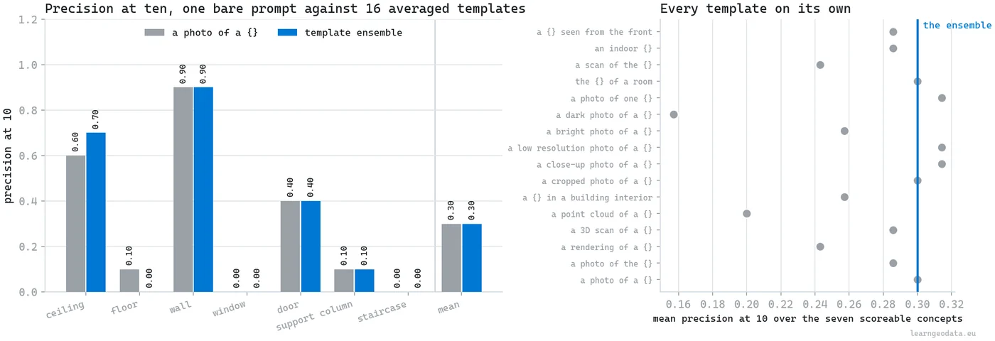
Now the scoreboard. On a real indoor test floor, precision at ten came out at 0.90 for “a photo of a wall”, 0.60 for ceiling, 0.40 for door, then 0.10 for floor, 0.10 for a support column, and 0.00 for window and for staircase. Three of the ten phrases queried, radiator, ceiling light and whiteboard, match no class anywhere in this survey, so a zero for them would score my vocabulary rather than the model, and they get reported as unscoreable probes. Every cosine in the run sits between 0.139 and 0.330, and the spread inside one concept averages 0.138, so compare regions within one prompt and never prompts within one region.
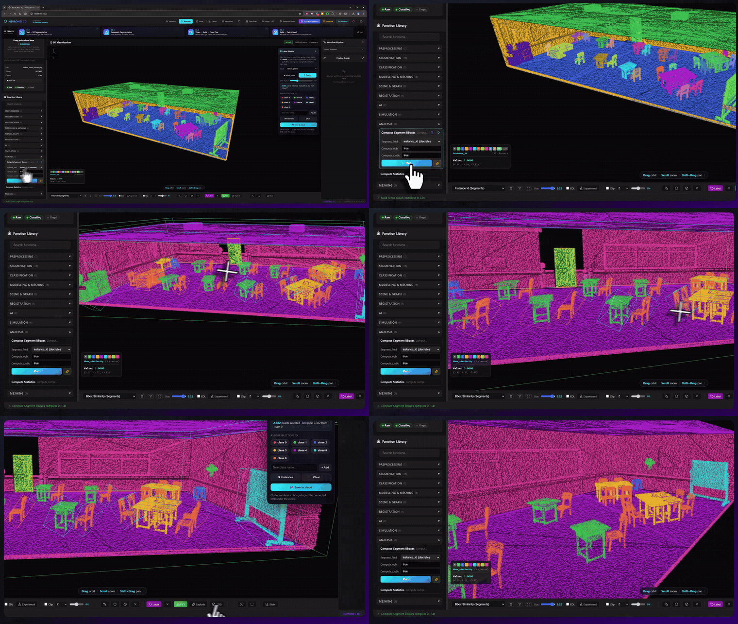
Where does this go when the retrieval side is taken seriously? OpenIns3D builds a far more careful snap-and-lookup version of the renderer above, and open-vocabulary 3D semantics in Python walks the practical version end to end.
How to Evaluate Multimodal 3D Models Honestly
An honest evaluation of multimodal 3D models splits by building rather than by region, and it costs you reported accuracy. Teach a head 1,454 regions from one floor, then score a different floor with a different layout and a staircase that never appeared in training, and you land on 0.654 accuracy with 0.558 macro F1 across 1,603 regions. A shuffled split hands back a prettier number and tells you nothing about the next site.
Then audit where your filters are allowed to run, because that is where this pipeline was quietly cheating itself. Candidate regions carry a purity score computed from ground-truth labels, and anything under 80 percent used to be dropped from both splits. On the training floor that is honest housekeeping, since you own those labels by definition and a region that is 60 percent wall and 40 percent window teaches a contradiction. On the test floor it means picking your exam questions after reading the answer key. The cut now runs on the training split alone: all 1,624 test regions get rendered and embedded, 1,603 of them get scored, and the 21 carrying a stair-flight code the head was never taught are reported separately rather than counted as errors it had no way to avoid.
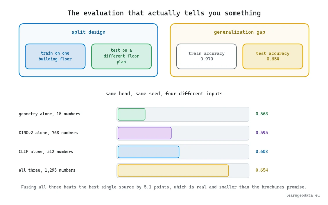
That correction costs 3.6 points of accuracy and 2.6 of macro F1. Where the leaky version printed 0.691, the clean one prints 0.654, and not one weight changed between them. If you find a filter of your own touching the test split, delete it and republish the lower number, because on a live scan nobody computes a purity score for you.
Then ablate every source of evidence with the same head, seed and epochs. Geometry alone, 15 numbers, reached 0.568. DINOv2 alone, 768 numbers, 0.595. CLIP alone, 512 numbers, 0.603. All three concatenated, 0.654. Retrain each row under eight head seeds and it shifts by 0.003 to 0.007, so treat any two rows within a point of each other as the same row.
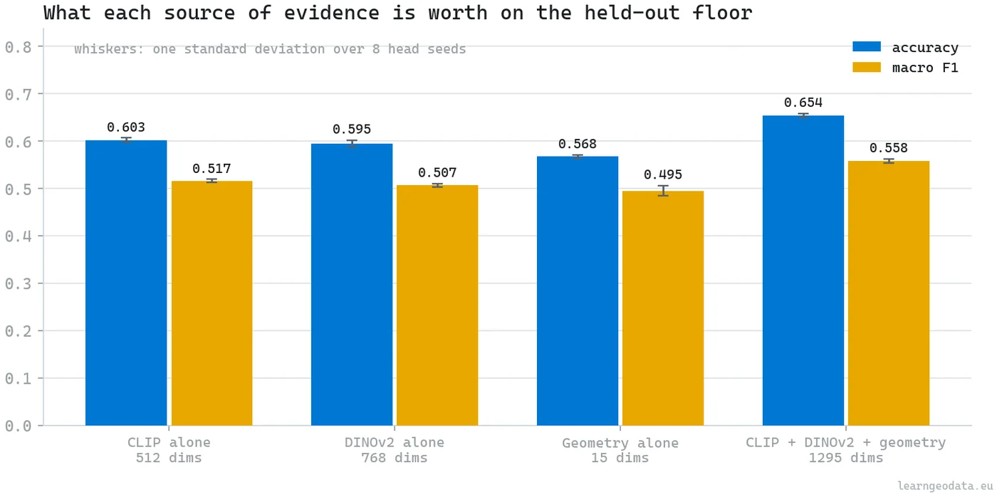
Three things there deserve an argument. Fifteen hand-written numbers landed within 3.5 points of a 151 million parameter vision transformer. The two backbones finished almost level despite completely different training objectives, so both are probably picking the same coarse shape out of these renders. And the fused run cleared the strongest single input by 5.1 points, which is a genuine gain and a much quieter one than fusion marketing implies.

Report accuracy and macro F1 together, and average macro F1 only over classes present in the ground truth, otherwise an absent class contributes a silent zero. Then put a second figure beside it. Restrict the average to the four classes backed by a hundred or more test regions and macro F1 reads 0.751 rather than 0.558, and the distance between those two is a statement about sample sizes rather than about the model. Beam or ledge had sixteen training regions. Keep recall and precision separate too: the window class hit 0.909 recall at 0.192 precision, and quoting either one alone would be a different kind of lie.
One check sits upstream of every per-class number here. The codes in this survey arrived as undocumented integers, so the names were read back out of measured geometry, and a name is a claim that deserves a number of its own. Resample each code’s objects with replacement four hundred times, rerun the naming rules, and eight of the nine readings come back identical every time. Clutter does not. It survives 0.65 of the resamples, and only 0.56 of its objects land nearest their own code’s median against a chance of 0.11. That is arithmetic telling you clutter is a bag rather than a class, so read any clutter score as a score about the bag.
🪐 System Thinking Note: Train accuracy was 0.970 and test accuracy 0.654, a 32-point drop. That gap is not a bug to be tuned away, it is the price of a split that mirrors deployment. Any evaluation design that shrinks the gap without changing the model has made your report prettier and your product worse.
Where Multimodal 3D Pipelines Go Wrong
Multimodal 3D pipelines go wrong inside one block of the confusion matrix rather than everywhere at once. On the held-out floor, ceiling scored 0.88 and floor 0.92 on the diagonal, while wall, door, window and column traded their errors with each other and with nothing else.
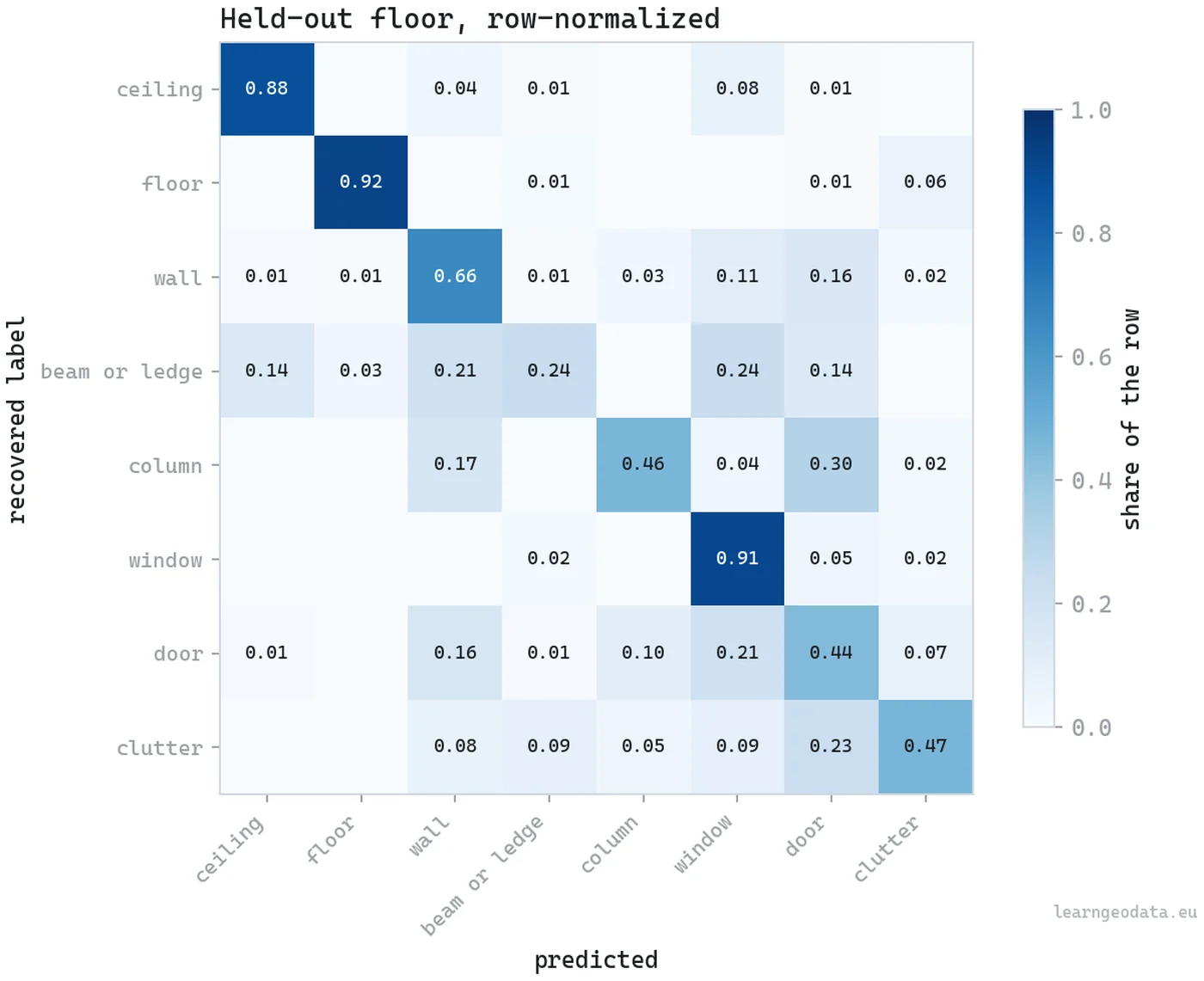
An accuracy figure tells you how often the answer came back correct. It says nothing about whether the errors are noise or one systematic blind spot you are about to ship, and those two need completely different responses. On the indoor run, the four commonest errors were wall called door 120 times, wall called window 85 times, door called window 52 times, and door called wall 41 times. All four sit between vertical planar surfaces, and none touches the ceiling or the floor. A blind spot you can point at physically is the good kind of bad news.
Confidence is the second trap, and it is the one where the softmax stops deserving your trust. Mean confidence when the model was right came in at 0.908. When it was wrong, 0.769. The distance between those two is real and you can act on it, and it is nowhere near wide enough to hang a safety threshold from. 193 wrong calls came back above 90 percent confidence, and the proudest mistakes were all one error: a narrow dark band in a pale wall, called a window at full confidence, because that is the appearance the model learned for “window”.
🌱 Growing Note: Write the verification layer next, and write it in geometry rather than in probability. A predicted window has to clear two tests: a sill somewhere in the 0.55 to 1.15 metre band, and a median brightness under the surrounding wall’s. A predicted column has to fit inside a 0.9 metre square footprint. You already know these thresholds, because they are how you would recognize the classes by eye, and none of them reads a label, so they stay legal at inference time. Run over the held-out floor, those two rules decline 199 of 1,603 calls, 164 of which were wrong and 35 right, lifting accuracy on everything they do answer from 0.654 to 0.722 and cutting the error count from 554 to 390. Giving up an eighth of the answers to remove nearly a third of the errors is a trade a client can weigh.
Five Multimodal 3D Mistakes and How to Fix Them
Five mistakes account for the distance between a multimodal 3D pipeline that demos well and one that survives a second building, and each of them shows up as a number rather than as an error message.
Letting a Filter Touch the Test Split
A purity filter computed from ground-truth labels used to drop low-purity regions from both splits here, and dropping them from the test split is choosing your exam questions after reading the answer key. The fix is to run the cut on the training split alone and republish the lower number. It cost 3.6 points of accuracy, 0.691 down to 0.654, with not one weight changed.
Cutting Regions After Choosing a Backbone
A foundation model names things, and a point cloud holds no things until somebody cuts it into some, so the segmentation decides the ceiling every backbone underneath it is measured against. A region that is 60 percent wall and 40 percent window can never be scored correctly no matter which encoder reads it. Fix the cut first, then argue about weights.
Cropping the Neighbours Out of the Frame
Rendering each region in isolation looks tidy and destroys the only evidence that separates a bare patch of wall from a bare patch of door. Leaving a pale ring of neighbouring points in the frame is worth 1.5 points on the full descriptor and 4.5 points on CLIP alone, which is a larger effect than every camera-placement decision in the rig combined.
Reading the Softmax as a Confidence
Softmax output is a ranking, not a probability of being right, and treating it as the latter is how a bad call reaches a deliverable. Mean confidence was 0.908 on correct answers and 0.769 on wrong ones, close enough that 193 wrong calls still cleared 90 percent. Pair it with a geometric check that reads no label, and accuracy on the answers you keep goes from 0.654 to 0.722.
Shipping Without a Geometry-Only Baseline
A fused descriptor that never gets compared against plain measurement is an unfalsifiable claim about your backbones. Fifteen hand-written numbers reached 0.568 on the held-out floor, within 3.5 points of a 151 million parameter vision transformer, so if your fused model cannot clear that line by a comfortable margin, the GPU is not earning its place in the pipeline.
Where to Go Next With Multimodal Foundation Models
Multimodal foundation models are one stop on a longer route that runs from raw sensing through to reasoning over whole scenes, and that whole route lives in the 3D Spatial AI with Python complete guide.
Two clicks sit either side of this one. Upstream are clean region proposals, the subject of 3D point cloud segmentation and clustering in Python. Downstream are the relationships between named regions, which semantic and spatial AI with scene graphs in Python picks up. Prefer to train the encoder rather than borrow one? 3D deep learning in Python covers that road instead.
For the scarcity argument made from the research side, GreenPLM is worth an hour, alongside a bias-controlled study of point clouds and spatial reasoning which finds that 3D input helps a language model without fixing its spatial reasoning.
If you want the same borrowing argument worked end to end on video rather than on a static archive, I wrote Turn video into smart 3D models, the Python guide with SAM, CLIP and DINO on Medium, where three frozen backbones are stacked into one pipeline and each is asked to do only the job it is good at. The rest of my Medium writing sits at medium.com/@florentpoux.
Run Your First Multimodal 3D Experiment This Week
Your first multimodal 3D experiment fits inside one afternoon. Pick a scan off your own drive, cut it into rough regions, photograph each from five directions with a ring of its neighbours left in the frame, run the frames through a backbone you paid nothing for, and fit a two-layer head on whatever labels you can assemble.
Then do the part nearly everyone skips. Read the confusion matrix, find the systematic mistake, and write the geometric rule that catches it. That rule is your product. The weights improve every year without you, and the check sitting on top of them is what a client cannot download.
Expect a modest number at the end of it. Mine was 0.654 on a floor the model had never seen. An earlier version of the same pipeline let a purity filter touch its own test set and reported 0.691, and those extra 3.6 points are the one thing here I would refuse to put in front of a client.
For a first real 3D Python task to run tonight, the free mission hands you one, and the Open3D repository is the reference you will keep open beside it. When you want this taught in order, with the parameter intuition and the failure catalogue no single article can carry, the 3D Spatial AI Program is where I teach it end to end.

Linnaeus did not discover a single new plant with his naming system. He made every plant anybody else found suddenly comparable. So which half of your pipeline are you going to name first, the borrowed half or the one nobody else can build?
Frequently Asked Questions About Multimodal 3D Models
Can You Use CLIP Directly on a Point Cloud?
Not directly, because CLIP reads pixels and a point cloud has none. You bridge the gap by cutting the scan into candidate regions, rendering each to a few images, then encoding those with the frozen tower. What you allow into the frame decides more than the camera positions do: on one indoor run, the pale ring of neighbouring points left around each region bought CLIP 4.5 points of accuracy on its own, and moving the cameras from surface-relative to world-axis positions changed nothing outside the seed noise.
How Many Labels Do You Need to Adapt a Foundation Model to 3D Data?
Far fewer than training from scratch. A linear probe on frozen embeddings trained usefully on 1,454 labelled regions from one building floor, moving 333,832 parameters against 238 million frozen ones in 0.19 seconds. Below a thousand examples, expect noisy per-class numbers. Above tens of thousands, test low-rank adapters instead.
Are There Foundation Models Trained Natively on 3D Data?
Yes, and they keep improving, but paired data limits them. Point-Bind maps a point encoder into CLIP’s space, and PointLLM bolts a language model onto that. Captioned 3D shapes number in the low millions against billions of image and text pairs, so these models lean on synthetic objects and transfer unevenly to cluttered scans.
Should You Combine CLIP and DINOv2 or Pick One?
Combine them, but expect a modest gain. On the same head, seed and split, CLIP alone reached 0.603 accuracy, DINOv2 alone 0.595, geometric descriptors alone 0.568, and all three concatenated 0.654. That is 5.1 points over the best single source, worth having and smaller than fusion is usually sold as.
How Do You Know When to Trust a Multimodal 3D Prediction?
Not from the softmax alone. On a held-out floor, mean confidence was 0.908 when the model was right and 0.769 when wrong, and 193 wrong calls came back above 90 percent confidence. Pair the score with an independent geometric check, such as requiring a predicted window to sit between 0.55 and 1.15 metres. Run as an audit on that floor, two such rules declined 199 of 1,603 calls and lifted accuracy on the rest to 0.722.
What Should You Install to Build This?
The stack stays small. open_clip supplies both towers and the tokenizer, PyTorch runs them, Open3D handles the point cloud and the offscreen renderer, NumPy carries the descriptors, and scikit-learn covers the standardization and the head if you would rather not write one.

