Julia Tutorial for 3D Data Science

Discover the make-it-all alternative to Python, Matlab, R, Perl, Ruby, and C through a 6-step workflow for 3D point cloud and mesh processing.

If you are always on the lookout for great ideas and new “tools” that make them easier to achieve, then you may have heard of Julia before. A very young language that is less than ten years old 👶, and that is a super cool way to get into fast scripting/coding for quickly achieving working ideas 🌼.

Supposing you are into scientific computing, machine learning, data mining, 3D data science, large-scale linear algebra, distributed and parallel computing, I think it is worth following up on this hands-on tutorial to get started with Julia and start doing fun 3D stuff!

In this newcomer tutorial, I will cut straight through the matter and provide you with a laser-focused 6-step workflow to get up and running with 3D data within the next ten minutes! Ready?

A bit of history?

Ha, but before, I want to highlight the ambitions of the creators of Julia. The creators of Julia, namely Jeff Bezanson, Stefan Karpinski, Viral B. Shah, and Alan Edelman. They blogged in 2012 about their aspirations and essentially why they initiated the Julia movement:

We want a language that’s open source, with a liberal license. We want the speed of C with the dynamism of Ruby. We want a language that’s homoiconic, with true macros like Lisp, but with obvious, familiar mathematical notation like Matlab. We want something as usable for general programming as Python, as easy for statistics as R, as natural for string processing as Perl, as powerful for linear algebra as Matlab, as good at gluing programs together as the shell. Something that is dirt simple to learn, yet keeps the most serious hackers happy. We want it interactive and we want it compiled. It should be as fast as C.

But do these claims hold 🤔? Is this an “I want it all” language? Well, I first discovered Julia in early 2019, when I was making a research visit to the Visual Computing Institute (Computer Graphics) in RWTH Aachen University (Deutschland).

Unsupervised Segmentation of Indoor 3D Point Cloud: Application to Object-based Classification
Florent Poux, Christian Mattes, Leif Kobbelt 3D GeoInfo Conference 2020 Point cloud data of indoor scenes is primarily…www.vci.rwth-aachen.de

Since then, I swear almost essentially through Julia! And that comes from a Pythonista/C “programmer” mindset. It is super clear, effortless to pick up, super-fast, and you can loop python scripts within, call your favorite libraries directly, and pure Julia will execute crazy fast! Indeed, Julia is compiled, not interpreted. For faster runtime performance, Julia is just-in-time (JIT) compiled using the LLVM compiler framework. At its best, Julia can approach or match the speed of C, and that is awesome 🚀! In three words, I would say that Julia is Fast, Dynamic with Reproducible environments.

⚠️ A warning, though, at the time of the writing, the documentation and tutorials are still very sparse, and the community is also pretty small compared to what you would be used to if using Python. But hey, I intend to change that a bit. Shall we dive in?

Step 1: Downloading and Installing Julia

Okay, now that you have your coffee ☕ or teacup 🍵 next to you, ready to find our way into the fog, let us dive in! First, we need to download Julia from the official website: https://julialang.org/downloads/

Note: This tutorial is made with Julia version 1.6.2, 64bits using windows, but you can use any stable release, which should work (in principle 😉).

Install the pretty stuff once the executable is downloaded until you have shiny “software” ready for your beautiful hands!

Step 2: Setting up your Julia development environment

Julia supports various editors like VSCode, Atom, Emacs, Sublime, Vim, Notepad++, and IDEs like IntelliJ. If you like Jupyter notebooks, you can also use them directly with Julia. For this tutorial, I will show you my favorite three choices to choose from.

Julia with Jupyter Notebook

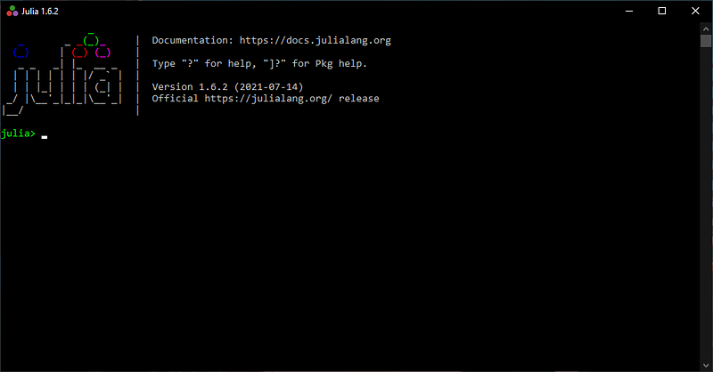
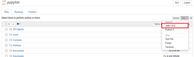
It would be the first choice to demo your project in a powerpoint-style fashion or if what you intend to do is more linked to an exploratory data analysis. For this, nothing simpler, launch your freshly installed Julia executable, then a window like below should pop up.

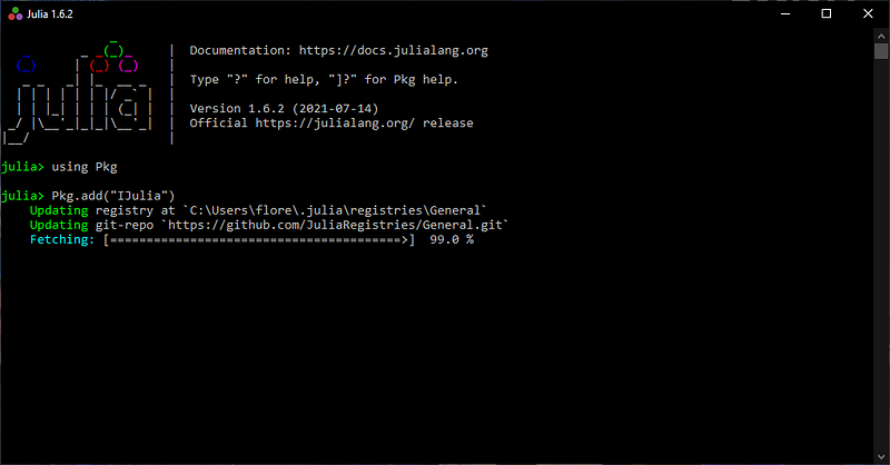
From there, all you have to do is to type the command using Pkg and then press Enter followed by the command Pkg.add("IJulia") and Enter. The process of installing the IJulia package necessary to use Julia within Jupyter Notebooks takes around 1 minute.

Then, you can launch Anaconda Navigator (with GUI) from which Jupyter Notebook on the environment of your choosing.

Note: If you do not have Anaconda installed, you can follow the tutorial below:

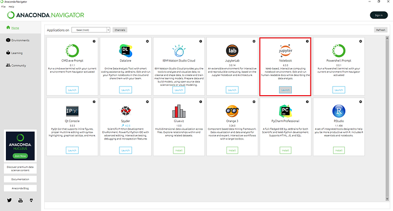
Once opened, you can create a new notebook with Julia acting as the programming language (see below for starting a new notebook)

Julia with Atom IDE and Juno

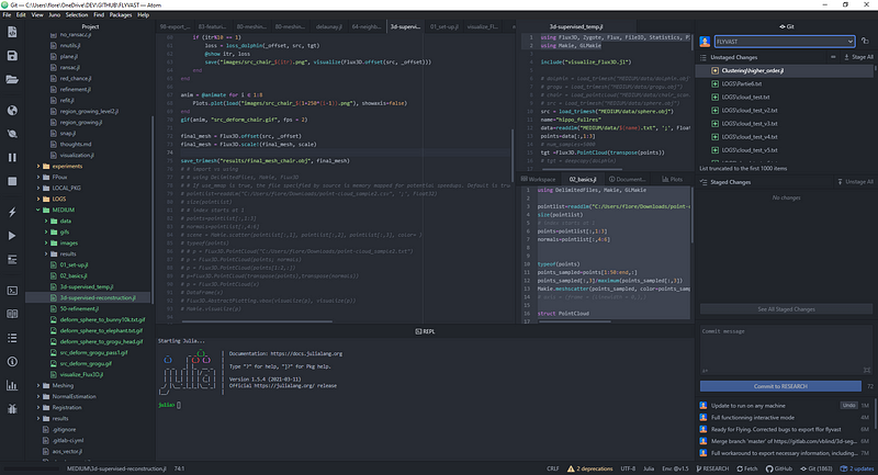
I tend to favor the Atom+Juno combination, which allows you to benefit from an interactive REPL mode, much like what you would be used to with Spyder. If you choose to follow in these footsteps, you first need to install Atom in your system following the instructions given at https://atom.io/.

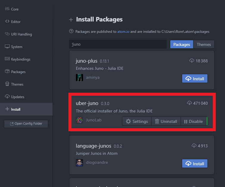
Then, you can launch Atom and head over to the package installation settings through Packages>Settings view>Open or the shortcut Ctrl+,. There search for juno and then click the install button for uber-juno and if not installed juno-client. Once Juno is installed, you can try opening the REPL with Juno > Open REPL or Ctrl+J Ctrl+O (Cmd+J Cmd+O on macOS), and then pressing Enter in the REPL to start a Julia session. And that is it! We are ready to code!

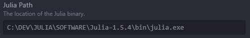
Note: If the REPL does not seem to launch correctly and does not display the Julia logo, head over to the Juno Client Settings from the Package menu and verify the path to tour Julia executable.

Bonus: Julia with Google Colab

You can also use a google Colab environment, but that needs a specific block of code to use Julia instead of Python. For this, you will find at this link a template that makes it possible to work directly within Colab. It also contains the main code of this tutorial.

Note: Every time you want to use Julia on the Google Cloud, you need to run the first block, refresh the page, and continue directly to the second block without re-running the first until every element is ready for you.

Step 3: Loading datasets

Great, so now we are ready to Julia code. First, let us discover where we are working, so our current working directory, using the command pwd(). Hmm, it looks like we are in the base directory, so let us change it to a project directory that you would create where you want to store most of your project (data, results, …) with cd(“C://DEV/JULIA/TUTORIALS/3D_PROJECT_1”), followed by pwd() to check out the new path.

Okay, we are all set. Let us download a dataset, for starters, a small noisy point cloud. For this, very handy, you can use the following command:

download("https://raw.githubusercontent.com/florentPoux/3D-small-datasets/main/tree_sample.csv","point_cloud_sample.csv")

Note: The download() command first takes the link to the data you want to download, which I dropped on my GitHub account, and then specifies its name locally after download.

Great, we now have a local version of the data in our working directory that we specified with the cd() command. Now, how do we load it in the script? well, we will make use of a Package called DelimitedFiles.

Note: A Package is a handy set of functions, methods, classes, and more that allow you to build on existing code without writing everything from scratch. The DelimitedFiles package allows manipulating (e.g., read and write) delimited files like our current point cloud at hand.

For using a package, we first have to load the package manager utility by just typing using Pkg. To add a new package, it is pretty simple; we just write Pkg.add(“DelimitedFiles”), and wait until the download + requirement checks are finished.

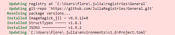
What is great about this is that you do not have to worry about dependencies (other packages needed by the current) as all is handled for you! Cool, huh? And on top, we can create excellent packages easily to ensure reproducibility of the results, for example, and independent environments, but that is for another tutorial 😉.

Note: Managing packages is then pretty straightforward, and we have a bunch of functions to update the packages, to know their current status, if we have any conflicts between them (rare), or to load unregistered packages by other like-minded coders, even one of your future local package 😉. I usually manage them by using the REPL and entering the package manager with the command ] in the right environment. To exit the package manager, one needs just to do Ctrl+C .

Ok, now that the package is installed (you only need to run this once per environment). You can use it in your current project by typing using DelimitedFiles, and also, if there are no conflicts of function names, you do not need to write from which package a function comes. to read a delimited file DelimitedFiles.readdlm() is equivalent to readdlm().

From there, let us read the point cloud at hand and store the data in the variable pointlist:

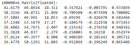
pointlist=readdlm(“point_cloud_sample.csv”,’;’)

The first lines should look like below.

Step 4: First pre-processing operations

Okay, pretty cool up until now, hun? And now, let us see the first real surprise if you are used to other programming languages: indexing. You can try doing pointlist[0] to retrieve the first element. What are we getting? a BoundsError.

Haha, in Julia, indexes start at 1, so if you want to retrieve the first element (the X coordinate of the first point), you just input pointlist[1] that returns 41.61793137. A bit confusing at first, it is pretty handy and logical, at least from a scientific point of view 😅. So now, if you want to retrieve the first point, then you need to know that indexes work on the first axis (rows) first, followed by the second axis (column(s)), and so on. Thus, to retrieve the first point (first row and every column):

pointlist[1,:]

Very cool, and now, to get further, if we want to store the coordinates in the points variables and the normals in the normals variable, we just do:

points  = pointlist[:,1:3]
normals = pointlist[:,4:6]

Note: If you want to know the type of a variable, typeof() is what you are looking for. typeof(points)will display that we deal with Matrices, which are an alias of 2-dimensional arrays. Also Float64 is a computer number format, usually occupying 64 bits in computer memory; it represents a wide dynamic range of numeric values by using a floating radix point. Double precision may be chosen when the range or precision of single-precision (Float32) would be insufficient.

One last straightforward pre-processing step would be to know how to quickly sample the variable extracting, let say, 1 line every tenth. For this, we can do the following (a bit like Python, but we need to put the word end to treat the total variable):

points_sampled=points[1:10:end,:] 

We first work on rows, taking one every tenth, and for each line, we keep all columns with : following ,.

Hint: There are many ways to sample a dataset, but it is always important to balance the gain performance/results. This way is pretty quick and straightforward to execute; thus, it usually acts to get first visual results to know what we are dealing with without using too much memory.

Step 5: 3D Data vizualisation

We now are ready to address 3D data visualization, a critical step to grasp what we are dealing with! Here, one library is the go-to solution: Makie. Because we didn’t use it yet, we first need to import the package, along with two other “backends” depending on your paradigm (webGL visualization or OpenGL visualization), namely WGLMakie and GLMakie. Nothing more straightforward, we just run the following three lines only once:

Pkg.add(“Makie”)
Pkg.add(“WGLMakie”)
Pkg.add(“GLMakie”)

Note: Once executed, if anytime you want to explore the packages you have installed in your current environment, you can use the command Pkg.installed().

Once the needed packages are installed, to make them usable in your working session, you can add the line using Makie, GLMakie (or using Makie, WGLMakie if you want interactivity on the web with Colab or Jupyter), much like import matplotlib in Python.

Nice, now, before visualizing, let us prepare a bit of color for our colorless points, depending on their z-value. We will create a color vector the size of the sampled point cloud that will range from 0 to 1, depending on how close to the maximum value it is, by dividing each point:

zcoloring_scale=points_sampled[:,3]/maximum(points_sampled[:,3])

Hint: Julia automatically understands that you want to divide each element from points_sampled[:,3] by the maximum value with maximum() . Handy, huh? But it is a particular case of broadcasting, which in Julia, you just write by inputting a . before your function or mathematic symbol. If you do ./ here, you will get the same result.

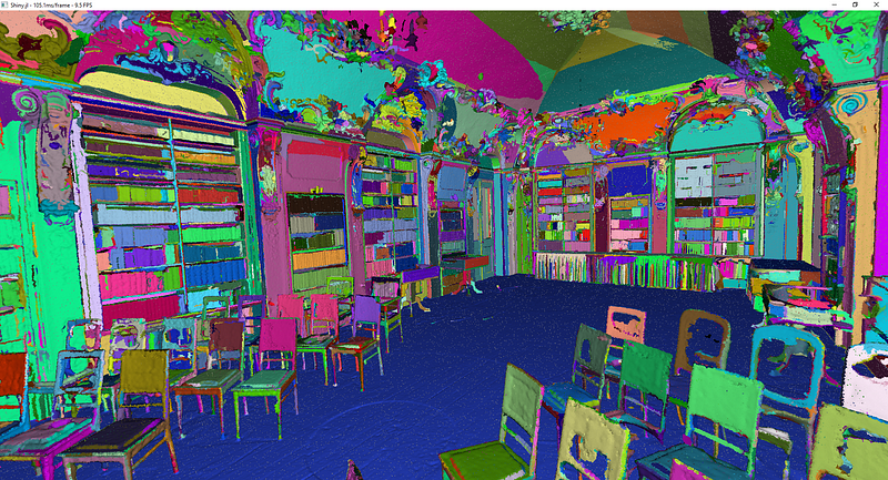
Okay, now, all we have to do is plot our results as a scattered point cloud in 3D. For this, we use the scatter function from Makie, and we pass as arguments the coordinates of the points (points_sampled), the color vector zcoloring_scale, and also some parameters like the size of each point with markersize, and if we want to display the axis.

scatter(points_sampled, color=zcoloring_scale, markersize=100, show_axis=true)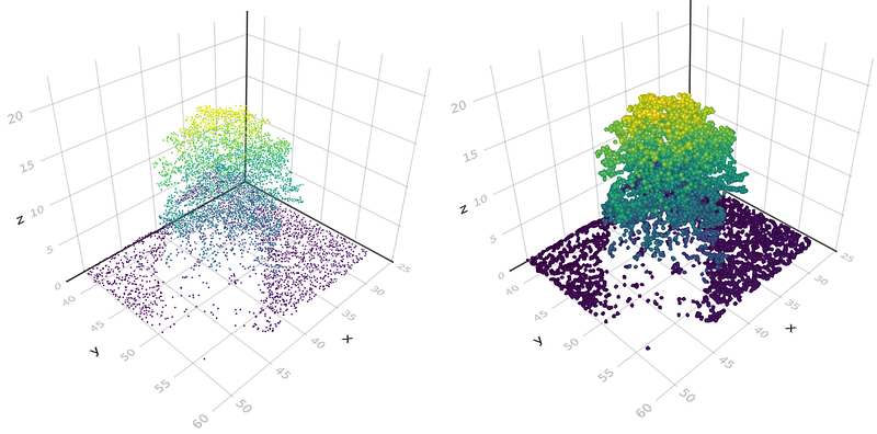

You also can do a meshscatter plot that will generate a small sphere for each point (like the image above on the right)

scene_1 = meshscatter(points_sampled, color=zcoloring_scale, markersize=0.2, show_axis=true)

How very cool! If you want some interactivity on the web, you should make sure to use WGLMakie instead of GLMakie, which will just give you a fixed backend to generate a view.

Hint: If you want to print your figure to a file, an effortless way is to first install the FileIO package using Pkg.add(“FileIO”) and using FileIO that holds the necessary methods and function to deal with a lot of file formats incl. meshes, images, vectors … Once available in your running session, a simple save(“scatter.png”, scene_1) will save the plot to an image in your working directory.

[BONUS] 3D Mesh I/O

An effortless way to display a mesh is to use FileIO, like hinted above. In two simple lines, you can display your mesh. Take the one available on my GitHub like the point cloud before with:

download("https://raw.githubusercontent.com/florentPoux/3D-small-datasets/main/hippo_1k.obj","hippo_1k.obj")

and then, you can just store it in the obj variable with:

obj = load(“hippo_1k.obj”)

that you pass to the Makie.mesh() function shortened to mesh() to display your 3D model.

mesh(obj, color=”honeydew2”, show_axis=false)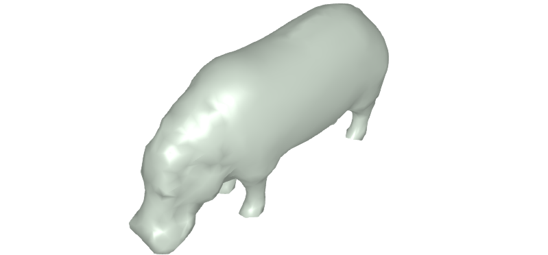

If this is not optimized code clarity, I do not know what it is 😆!

Hint: If you want to access the single-shot color names, check out this link that gives all the available possibilities, and there are a lot 🙃.

Step 6: 3D Data Analysis

Now we can explore a bit the data and play around with some functions. The first thing would be to know how to access a specific portion of the 3D point cloud dataset. In our case, we would like to find and separate (more or less) the ground from the rest. First, we would find through visualization the higher z of the ground and then use that as a threshold. Let us plot the 2D projection of the dataset:

scatter(points_sampled[:,2:3], color=zcoloring_scale, markersize=100, show_axis=true)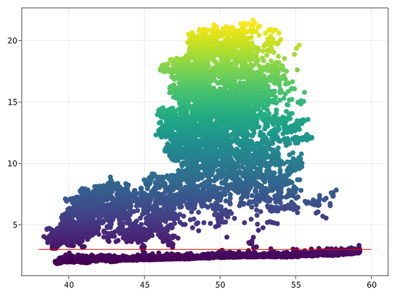

We can identify that we get a threshold at more or less 3 meters (red line). Let us use it directly for our experiments.

Hint: If you want to display other elements on the same figure, a simple way to do is to add ! to the following plots, like if you want to display the y=3 line in red like above, you would do lines!(range(38, 60, length=30),(x*0).+3, color=”red”) and admire the results with the commandcurrent_figure() 😀.

Now we want to find all points below and above the visually defined threshold and store them in a separate variable. We will use the findall function that returns the indexes of the points satisfying the condition in brackets. Let us work solely on points[:,3] as we just need to study this and retrieve indexes that we can later use to filter our full point cloud. How cool 😆?

indexes_ground=findall(x->x < 3, points[:,3])
indexes_tree=findall(x->x>=3, points[:,3])

Very nice! Now, if we would like to get the points corresponding to these indexes list, we just have to pass indexes_ground or indexes_tree as a row selector in the points variable, for example, for getting all the points that belong to the ground and all the rest. And if we want to plot this, then we can do:

meshscatter(points[indexes_ground,:], color=”navajowhite4”, markersize=0.3, show_axis=false)
meshscatter!(points[indexes_tree,:], color=”honeydew3”, markersize=0.3, show_axis=false)
current_figure()

Awesome! We just did a manual instance segmentation step, where we have one ground element and one tree element, and that with a new language; well done!

Conclusion

In Julia, you just learned how to import, sub-sample, export, and visualize a point cloud composed of hundreds of thousands of points! Well done! But the path does not end here, and future posts will dive deeper into point cloud spatial analysis, file formats, data structures, visualization, animation, and meshing. We will especially look into managing big point cloud data as defined in the articles below.

This Article is derived from the one originally published in Towards Data Science