

Point cloud ingestion is the layer between any capture device and everything you do afterwards. It reads whatever container arrives, resolves the coordinate reference system, normalizes attribute names, and emits one record with stated units, a provenance trail, and an explicit list of what it could not determine. It processes nothing. Its only product is uniformity.
| What it is | A normalization layer that sits between any capture device and the rest of your pipeline |
| What you build | One ingestion function that returns a normalized record: stated units, a resolved coordinate system, a provenance trail, and an explicit list of the gaps |
| Libraries | laspy with the lazrs backend, pyproj, shapely, Open3D, NumPy, SciPy |
| Worked on | Four real captures: a national LiDAR tile, an aerial survey, an indoor mobile scan, and a phone capture |
| Level | Expert. Assumes Python and basic 3D geometry. |
So what happens when four captures disagree about units, position and precision, and every one of them insists it is right?
The guide runs in the order you would actually build this, starting from what arrives on disk and finishing with a footprint you can hand to somebody else. Here is the path:
- What Is Point Cloud Ingestion?
- Why Use One Ingestion Layer Instead of Many Readers
- How to Read a LAS Header in 1 Millisecond
- How to Resolve a Point Cloud Coordinate Reference System
- How to Normalize Point Cloud Attributes Across Sensors
- How to Measure Point Cloud Density Correctly
- How to Choose a Voxel Size and Emit a Footprint
- Five Point Cloud Ingestion Mistakes and How to Fix Them
- Build Your Point Cloud Ingestion Layer This Week
- Frequently Asked Questions About Point Cloud Ingestion
Something has shifted in how we build, and I suspect you have felt it too.
The tooling got wonderfully good. Code comes together faster than it used to, and I still love the craft of it.
What I find myself spending my best hours on is a different question: how do we make all of this work to the very best of our abilities?
That part is the science. Choosing the method, designing an approach that answers the question in front of you, then standing behind that choice when somebody asks why. It stays ours, and it is what this guide is really about.
Because capture is going everywhere. Phones, helmets, drones, site cameras, robots that map a floor while they clean it. Within a few years the buildings and roads around you carry a continuous 3D record.
Every claim anybody makes on top of that record rests on one small question: did somebody, at intake, write down what the data can and cannot support?
Nobody hands out awards for that layer. It still decides whether the rest of it is true.
Here is the encouraging part. This was solved once already, in a different century, for a different measurement.
What 1875 Teaches Point Cloud Ingestion
On 20 May 1875, delegates from seventeen countries signed a treaty in Paris about a bar of platinum, the metre des Archives. You can still read that treaty at the International Bureau of Weights and Measures.
Nobody invented a new length that day. They agreed on one physical reference that every signatory would defer to. Before it, a metre in Lisbon and a metre in Saint Petersburg were cousins rather than twins.
Now open a folder of point clouds. One file states its coordinate system where a parser can find it, one hides it in the filename, and one keeps quiet.
You are in the pre-1875 situation right now, and point cloud ingestion is the work of getting out of it.
What you will learn in this article
- What a sensor abstraction layer is, and why one normalized record beats a folder of import scripts
- How to read everything useful out of a LAS or LAZ file in about a millisecond, without decoding a point
- How coordinate reference systems, datums and the vertical question actually break in practice
- Why measured point spacing, taken in more than one place, decides which algorithms you can run
- The ingestion traps that produce files which open fine and are completely useless
What Is Point Cloud Ingestion?
Point cloud ingestion is the layer between any capture device and everything you do afterwards. It processes nothing. It turns whatever arrived into one agreed shape, so nothing further down your stack ever needs to know which sensor produced its input.
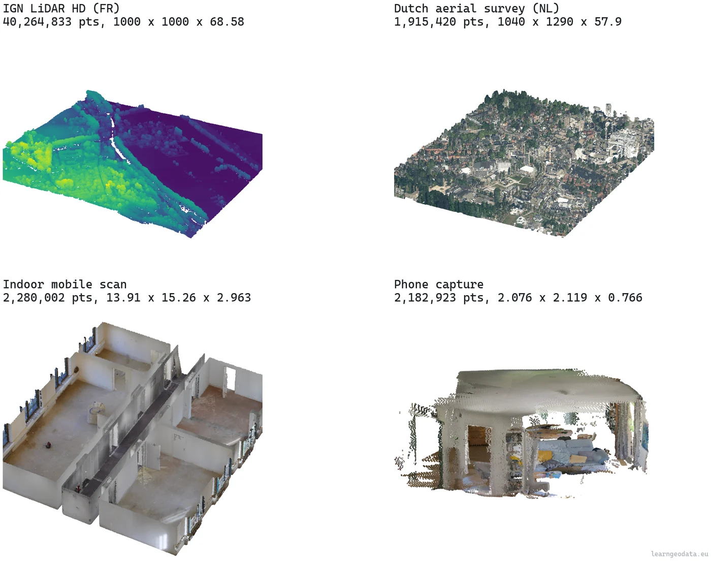
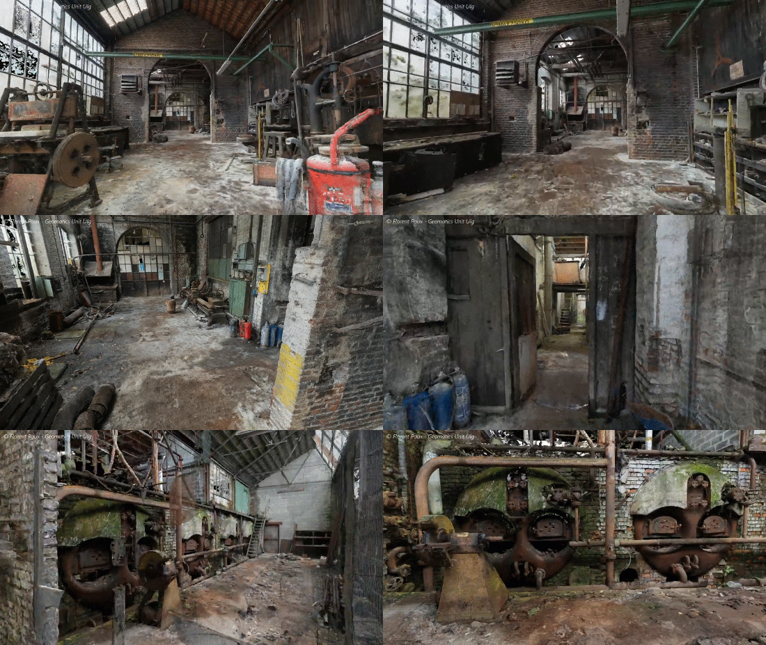
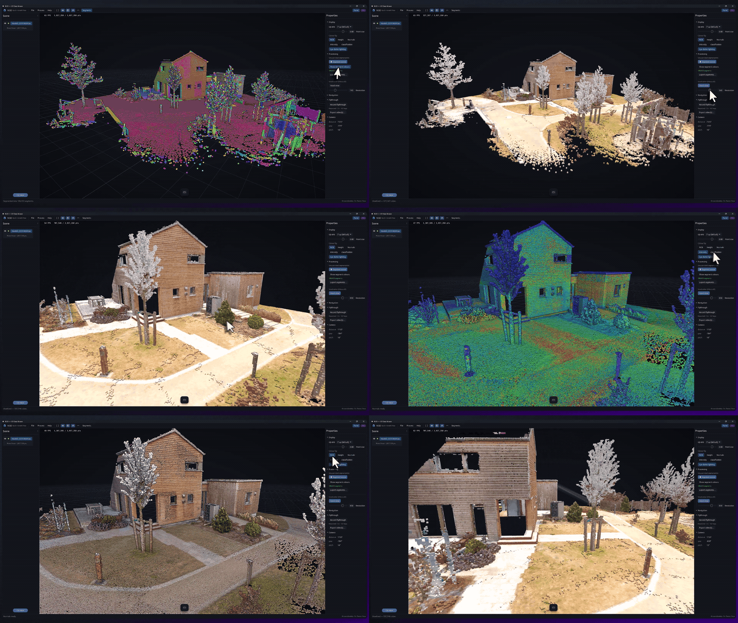
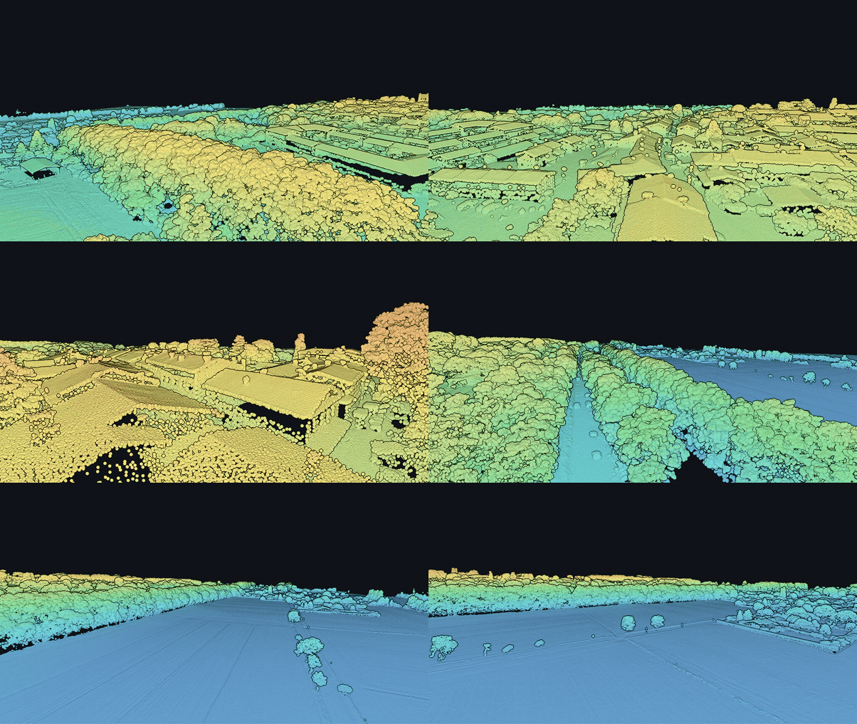
Here is a real week of arrivals: four captures from four different worlds.
Five compartments cover the record that comes out the other side:
- Geometry as float64, left in the frame the file used.
- Attribute channels flattened onto a vocabulary you fixed in advance.
- Declarations, so the coordinate system and the units arrive with a named source attached.
- Provenance, so anyone can retrace which reader ran, how long it took, with which seed.
- Gaps, which catalogue what the layer declined to decide.
Skip that fifth compartment and you pay for it later.
Say a file has no classification. A schema with nowhere to put an absence hands your model an array of zeros, and zero is a legal ASPRS code, so nothing anywhere raises a flag. A schema that can write “no classification in this capture, here is why” makes that mistake impossible to have.
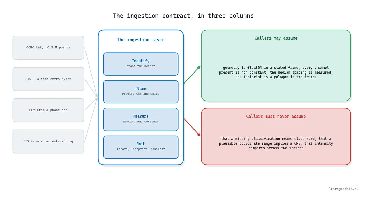
Notice what the contract refuses to promise. It never says the capture is georeferenced, only whether it is. Writing that distinction down is the entire discipline.
Why Use One Ingestion Layer Instead of Many Readers
You know how this goes.
A pipeline gets written for one dataset and works beautifully. Then a delivery lands from a different vendor. Duplicating the loader takes eleven minutes, generalizing it takes a day, so you duplicate. Four repeats later you own a directory nobody volunteers to open.
The reading code was never the expensive part. It is short and dull.
The expense arrives when your segmentation, meshing and training loop each grow a small branch that knows which loader ran, because sensor knowledge has nowhere else to live. No single branch looks wrong in review, which is why the coupling survives until it is load-bearing.
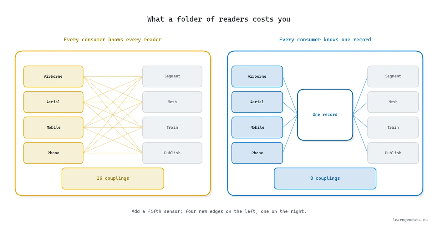
You can count the damage. Four readers talking straight to four consumers give you 16 pairings that can drift. Put one record in the middle and there are 8.
Add a fifth sensor: the direct arrangement grows by four, the layered one grows by one. That is the whole business case, whether your consumers are analysts or training runs.
Meeting a new sensor should cost you one small function and change nothing else you own. So where does that function start? Not with the points.
How to Read a LAS Header in 1 Millisecond
Decoding is the costliest thing you can do to a point cloud, and you can plan an entire job without it.
A small block of bytes at the front of the file carries the format and version, the row count, the extent, the scale and offset, every dimension name, and the coordinate system if the writer recorded one.
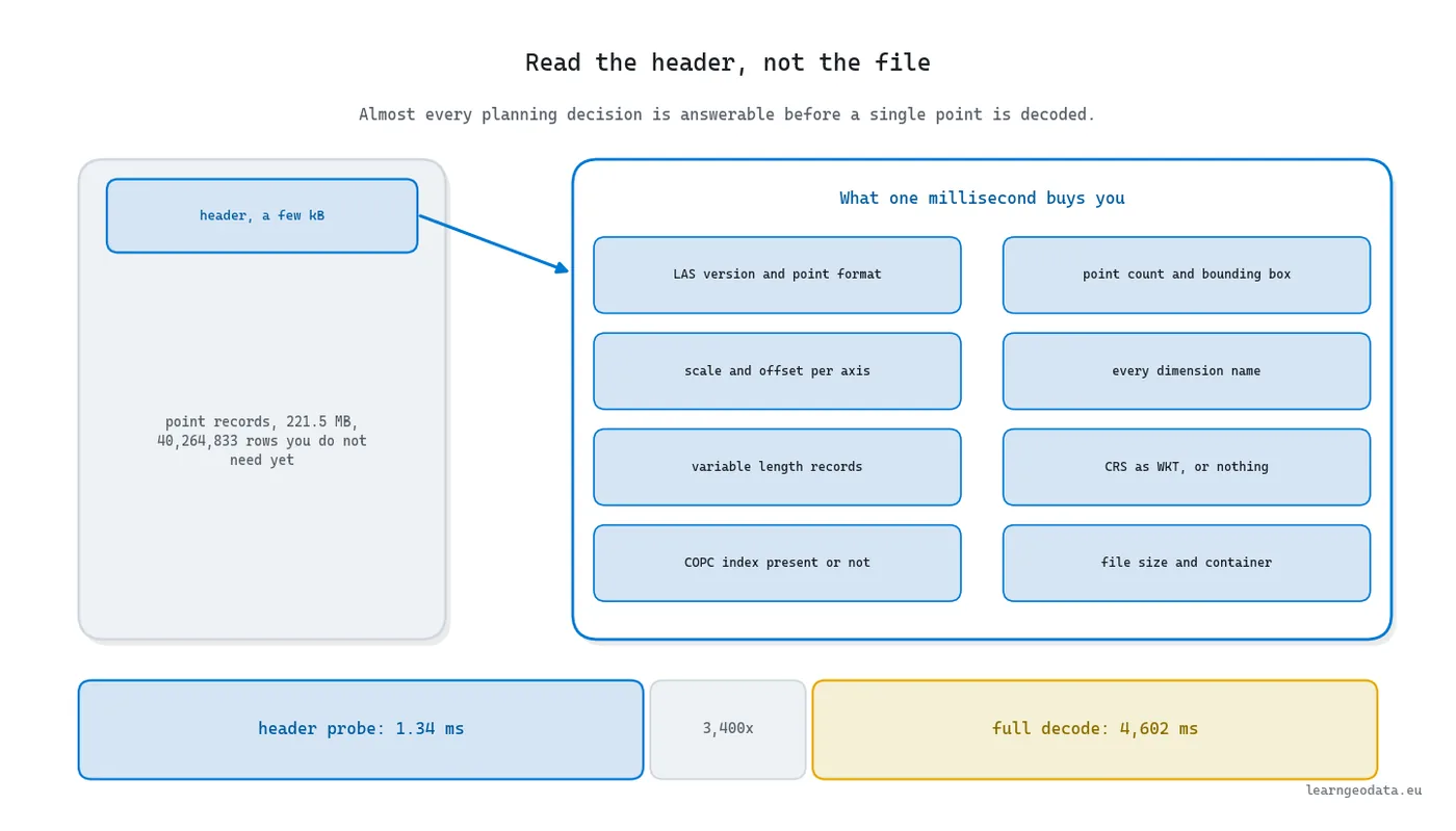
How much does skipping the decode buy you? An IGN LiDAR HD tile of 221.5 MB and 40,264,833 points gave up its whole header in 1.34 milliseconds. Streaming and decimating the same tile cost 4,602 milliseconds.
That is a factor of 3,400 between knowing what a file is and opening it, and your planning decisions come out the same either way.
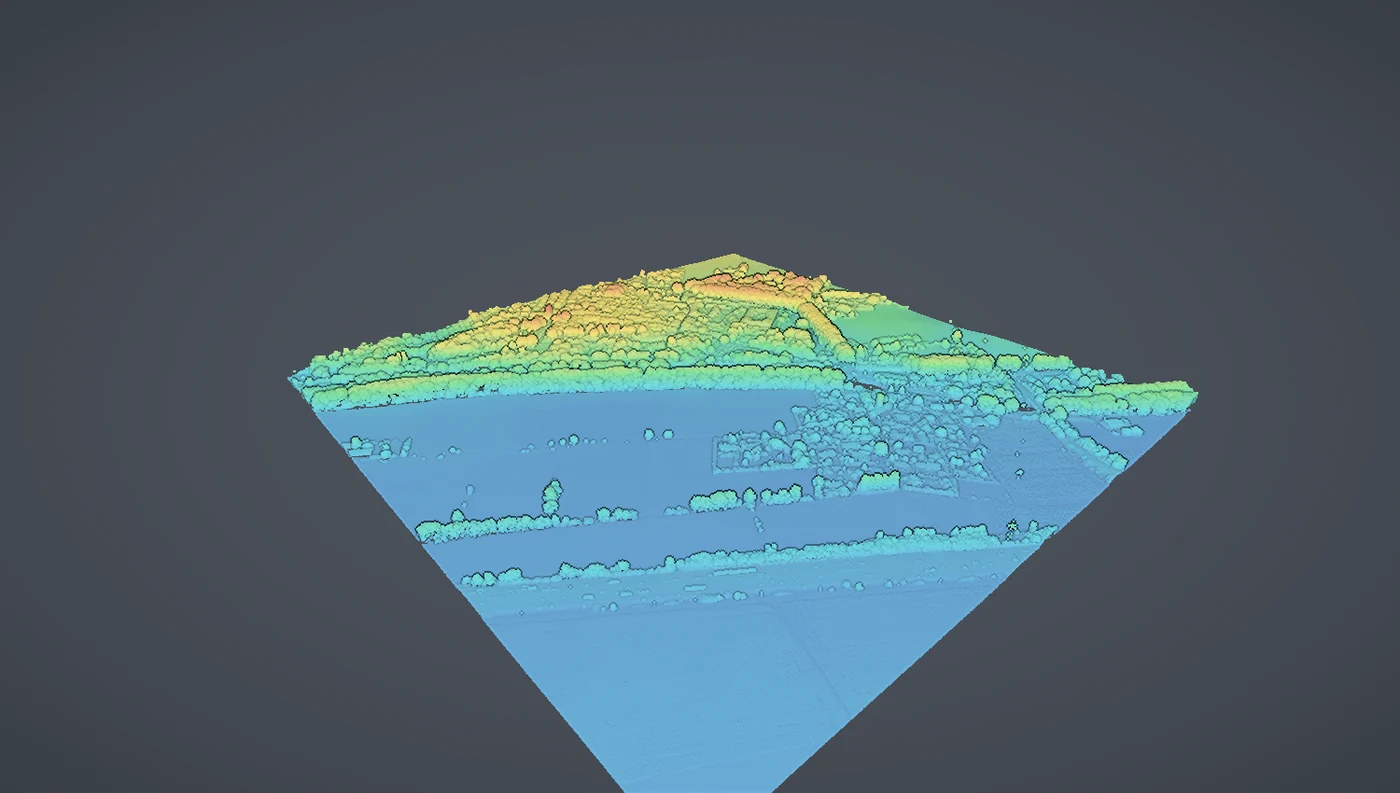
Put the function below at the top of any intake script. Opening a file through laspy inside a with block pulls the header and the variable length records and stops there, so no row is ever materialized.
Hand back a dictionary, not a class instance, because whatever leaves this function has to survive json.dumps on its way into a manifest. The parse_crs() call returns a pyproj object or None, and None is a finding rather than a failure.
import laspy


def describe(path):
    """Everything a LAS or LAZ file will admit to, in about a millisecond."""
    with laspy.open(path) as fh:
        head = fh.header
        crs = head.parse_crs()
        span = [round(hi - lo, 3) for lo, hi in zip(head.mins, head.maxs)]
        return {
            "points": int(head.point_count),
            "container": f"LAS {head.version} pf{head.point_format.id}",
            "extent": span,
            "scales": [float(s) for s in head.scales],
            "dimensions": sorted(head.point_format.dimension_names),
            "epsg": None if crs is None else crs.to_epsg(),
            "compound_crs": bool(crs is not None and crs.is_compound),
            "copc_indexed": any("Copc" in type(v).__name__ for v in head.vlrs),
        }


for name in ("airborne.copc.laz", "aerial.las", "indoor.las"):
    print(name, describe(name))
Run that across a real delivery and the arithmetic stops being an argument.
| Capture | Points | Header probe | Full decode |
|---|---|---|---|
| Airborne LiDAR HD (FR) | 40,264,833 | 1.34 ms | 4,602 ms |
| Aerial survey (NL) | 1,915,420 | 1.45 ms | 372 ms |
| Indoor mobile scan | 2,280,002 | 0.36 ms | 250 ms |
| Phone capture | 2,182,923 | 0.56 ms | 81 ms |
Keep the copc_indexed flag even if nothing uses it yet. Cloud Optimized Point Cloud files carry an octree, so a viewer can fetch the nodes covering a bounding box instead of dragging the whole tile across the wire. Build a tile service later and that one boolean decides your design. The COPC specification reads end to end in twenty minutes.
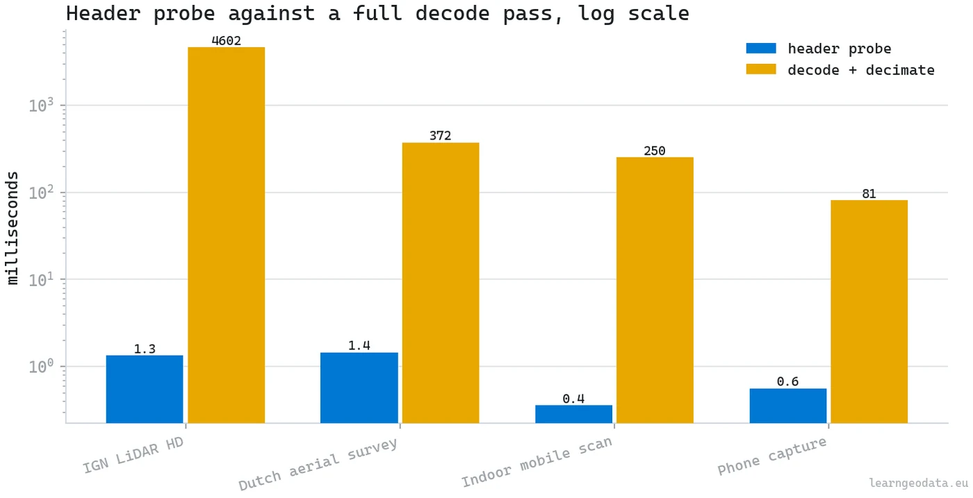
🦥 Geeky Note: If you benchmark this, run the probe twice and report the second timing. A cold first call measures whatever your operating system did with the file rather than your code. Warm, the four captures came in at 1.34, 1.45, 0.36 and 0.56 milliseconds. At that price you can probe a thousand-file delivery before committing an hour of processing to it.
Once you know what you have, the next question is the one that ruins careers.
How to Resolve a Point Cloud Coordinate Reference System
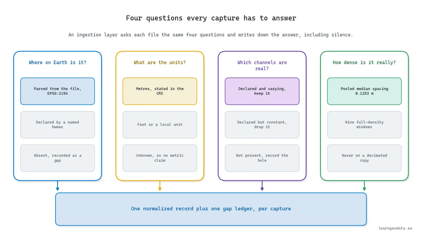
A point cloud coordinate reference system has only three honest answers when you ask a file where it sits. It told you itself. Somebody with a name told you. Nobody knows.
And here is where the 1875 story stops being decoration.
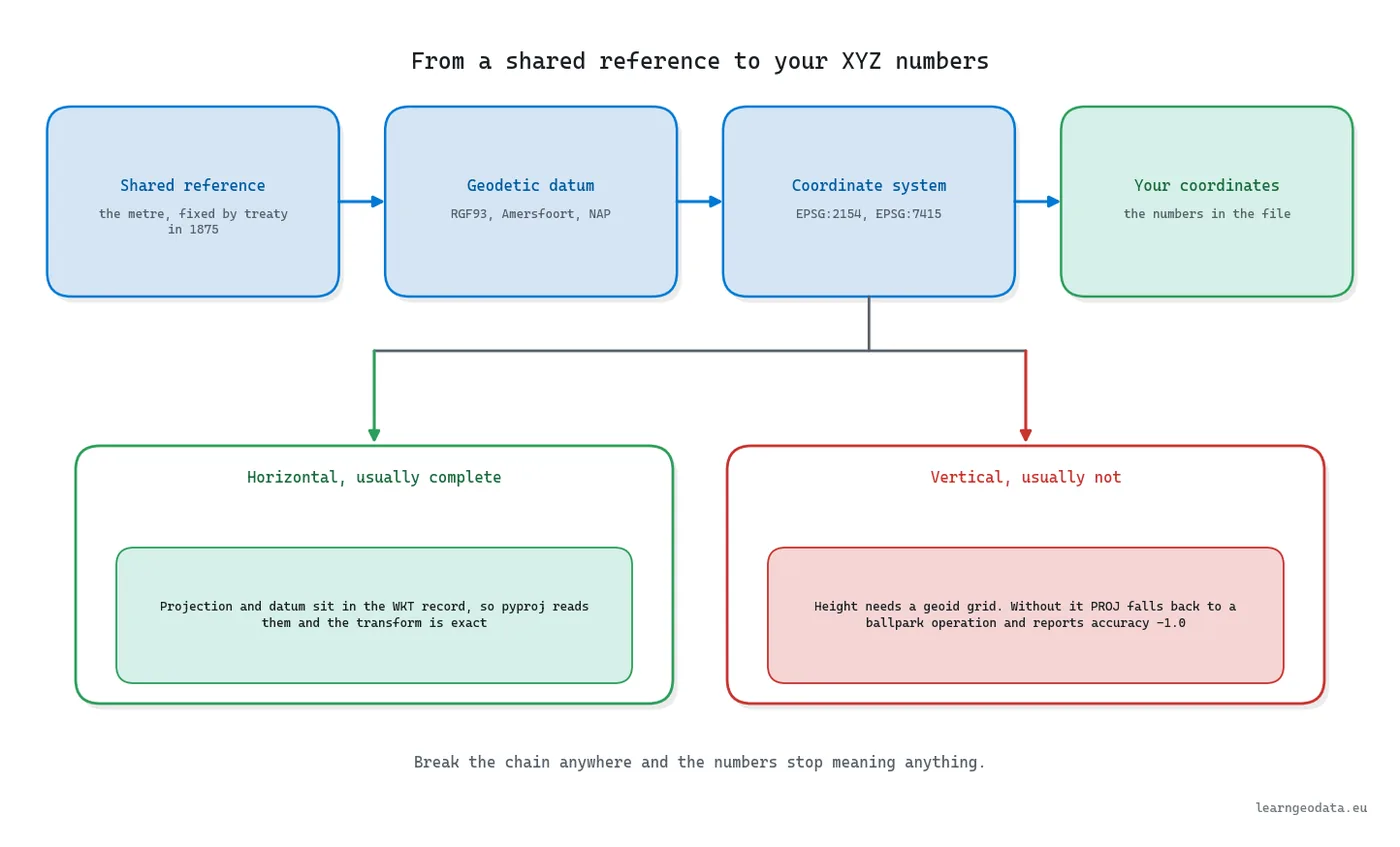
A coordinate reference system is what those delegates built: a chain from a shared physical reference, through a geodetic datum, to numbers that mean the same thing to two people who have never met. Break the chain anywhere and your coordinates are decimals.
Your code can produce a fourth: a quiet guess, made because the coordinate magnitudes look about right for a system you have met before. That habit does more damage than anything else in this trade. It never throws, never logs, and surfaces years later inside somebody else’s deliverable.
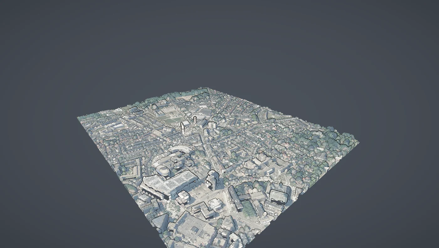
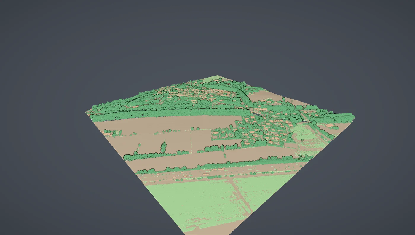
Of four real captures, two answered. A French tile parsed cleanly to EPSG:2154, Lambert-93. A Dutch aerial tile of the kind published by AHN parsed to EPSG:7415, a compound system pairing RD New horizontally with NAP height vertically.
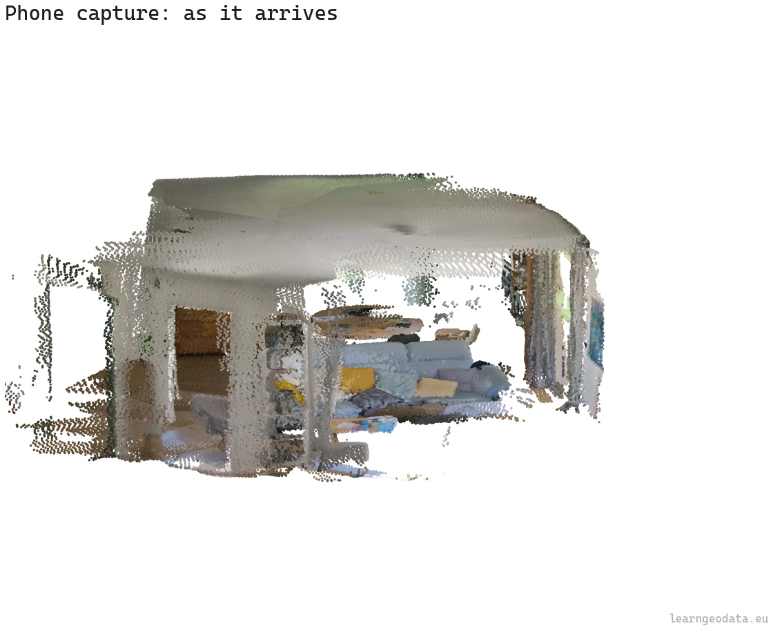
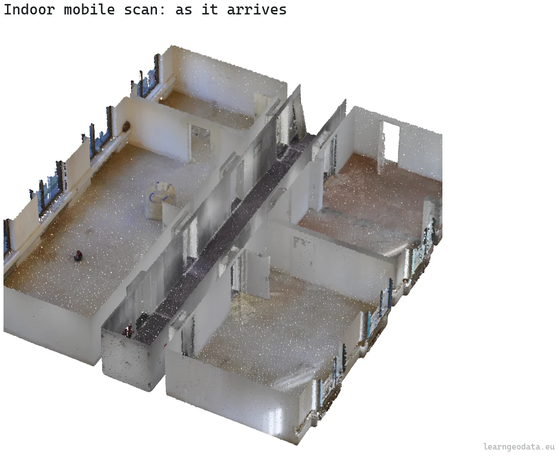
The other two said nothing. An indoor mobile scan of 2,280,002 points carried no coordinate system at all. A phone capture of 2,182,923 points was not even in metres, its bounding box measuring 2.076 by 2.119 by 0.766 of something.
🦚 Florent’s Note: Look at how national data ships and you will often find the vertical datum written into the filename, IGN69 in the French case, while the embedded record stays horizontal only. The height reference is legible to whoever downloaded the file and invisible to every tool that touches it afterwards. I would rather log that as an open question than proceed, because a pipeline confident about heights it never checked is worse than one that admits it does not know.
Two placeable captures need one shared frame, and I reach for EPSG:4978 over any projected system. Earth-centred earth-fixed metres are global with no zone edges to fall off, which matters when your tiles sit 1,051 kilometres apart. Keep the source coordinates too, since ECEF is miserable to work in locally.
import numpy as np
from pyproj import CRS, Transformer
from pyproj.transformer import TransformerGroup


def to_shared_frame(xyz, source_epsg, frame_epsg=4978):
    """Send a capture to one common metric frame, and price the round trip."""
    src, dst = CRS.from_epsg(source_epsg), CRS.from_epsg(frame_epsg)
    out = Transformer.from_crs(src, dst, always_xy=True)
    home = Transformer.from_crs(dst, src, always_xy=True)
    x, y, z = out.transform(xyz[:, 0], xyz[:, 1], xyz[:, 2])
    bx, by, bz = home.transform(x, y, z)
    residual = np.abs(np.column_stack([bx, by, bz]) - xyz).max()
    return np.column_stack([x, y, z]), float(residual)


def vertical_is_real(source_epsg):
    """Ask PROJ whether the height transform it would pick actually exists."""
    group = TransformerGroup(CRS.from_epsg(source_epsg),
                             CRS.from_epsg(4979), always_xy=True)
    best = group.transformers[0].description.lower() if group.transformers else ""
    absent = sorted({g.short_name for op in group.unavailable_operations
                     for g in op.grids if not g.available})
    return {"ballpark": "ballpark vertical" in best,
            "missing_grids": absent,
            "accuracy_m": group.transformers[0].accuracy if group.transformers else None}
Two details carry that snippet.
The always_xy=True argument stops pyproj honouring each system’s declared axis order, which is how people end up with coordinates in the Indian Ocean.
The round-trip residual is your receipt. The French tile returned a maximum error of 6.5e-09 metres. The Dutch tile returned 4.5e-04 metres, because its datum shift needs an uninstalled grid.
Run the second function before you trust any height. On the Dutch tile it reported 3 available operations, 2 unavailable ones and a missing geoid grid, with the preferred operation calling itself a ballpark vertical transformation and reporting an accuracy of -1.0.
PROJ will not raise. It passes your NAP height through as though it were ellipsoidal, and the cloud still sits convincingly on the terrain. Missing grids come from cdn.proj.org.

Two captures placed, two honestly unplaceable. That is a correct outcome, not a bug list. Now for what each file says it contains.
How to Normalize Point Cloud Attributes Across Sensors
Attribute naming is where every vendor asserts its own personality.
An airborne delivery gives you intensity, a classification code, return counts and a GPS timestamp. A survey-grade aerial tile adds colour, near-infrared and three RIEGL extra-byte fields. An indoor scan brings colour plus a custom instance dimension, and a phone brings colour alone.
Those dialects are not arbitrary. They fall out of how each instrument physically makes its measurement, unpacked device by device in 3D Scanning: Your Complete Sensor Guide.
Flattening those dialects onto a fixed vocabulary takes an afternoon. Nine names handle everything I have been sent: colour, near-infrared, intensity, reflectance, amplitude, class code, return pair, timestamp and instance identifier.
The interesting decision is not the naming. It is the gate you put in front of it.
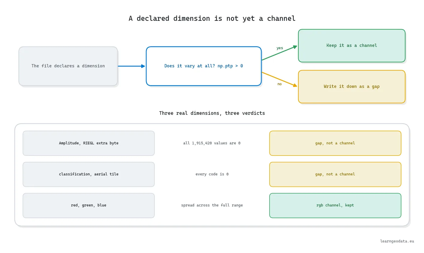
Here it is: promote a dimension to a channel only after you have watched it move. One call to np.ptp decides, and a peak-to-peak of zero sends the dimension to the gap list instead of into your record.
Real data makes the case. That Dutch tile declares a RIEGL Amplitude field whose 1,915,420 entries are identical zeros, plus a classification whose codes are identical zeros too. Trust the declaration and you have fed two constants into every statistic and model input downstream, where they will average, plot and train perfectly happily.
🪐 System Thinking Note: Notice what the 1875 delegates chose to standardize. They anchored the metre to an object you could walk up to and measure, not to a definition everybody promised to honour. Your channel vocabulary deserves the same treatment: describe what a capture demonstrably contains, not what its format allows it to claim. Applied across four files, that gate wrote 26 explicit absences, and a client would happily pay for those 26 sentences before assigning anyone to model the data.
Keep the raw values beside any normalized copy. Stretching intensity into a zero to one range makes it usable inside one capture and permanently unusable between two, which is the right trade for classification and the wrong one for anything calibrated.
Channels sorted, one number is left, and it is the one everything downstream leans on.
How to Measure Point Cloud Density Correctly
Density usually gets estimated by dividing the point count by the footprint area. That assumes the sensor spread its returns evenly. It never does.
Flight lines double the returns along their seams. A mobile trolley leaves a dense ribbon along its own path and thins towards the walls. Photogrammetry rewards texture and abandons blank surfaces.
What you want instead is the distance from each point to its closest neighbour, sampled in several separate places across the file and reported as a distribution rather than one figure.
A KD-tree makes that cheap. Ask each sampled point for its two closest matches, drop the first because a point is always its own nearest neighbour, then take the median with the fifth and ninety-fifth percentiles.
Here is where it goes wrong, and I walked straight into this myself.
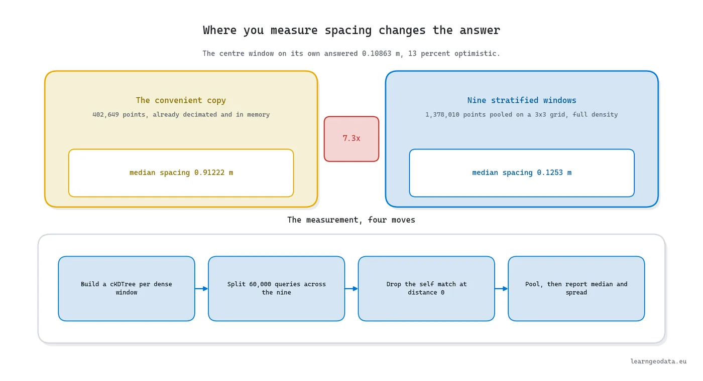
Your working copy is already thinned and already in RAM, so measuring on it saves two lines and several seconds. Do that on the French tile and the median comes out at 0.91222 metres. Measure at native density instead and the same code returns 0.1253 metres.
A factor of 7.3, biased towards making a perfectly good survey look too coarse for the job you meant to run.
Calling it an error understates it. The thinned number is a correct measurement of the wrong object: it reports how far apart your own samples landed, which is a fact about your stride, not the scanner.
Then there is the version of the same mistake that survives your first fix.
Reading one box back at full density is the obvious repair. Drop that box in the middle of the tile and you have traded a wrong answer for a local one. Split the plan extent into a 3 by 3 grid instead, put one box inside each cell, and pool what comes back.
On the French tile the nine boxes disagree by a factor of 1.59, and the middle box alone answers 0.10863 metres against a pooled 0.1253 metres. That is 13 percent optimistic, with nothing in its own output to warn you. The phone capture is worse: its windows range over a factor of 2.33 and the central box comes back 25 percent optimistic.
Ship the spread beside the median and a second signal comes free. Nine windows agreeing to within 10 percent is a uniform delivery. Nine windows disagreeing by a factor of two are telling you one number was never going to describe that capture.
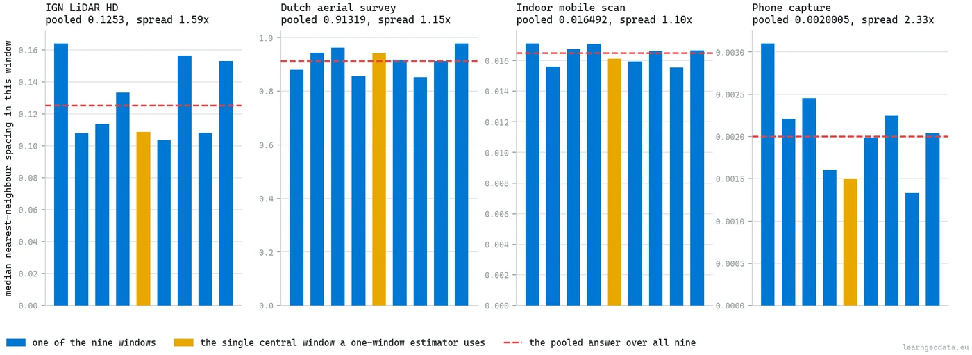
🦥 Geeky Note: Sixty thousand query points settle the median and still return in a fraction of a second once you hand scipy.spatial.cKDTree every core with workers=-1. Split that budget evenly between your windows, so each weighs the same regardless of how long the sensor sat over it. Strip out distances of exactly zero, and count them instead of dropping them quietly: 15.2 percent of the points sampled from the indoor scan sit exactly on top of another point, and no header in that file mentions it.
Now the payoff. Ask which captures can carry a 25 centimetre analysis cell, on the conservative rule that you want two independent measurements across a cell, and the French tile fails.
The shortfall is 0.3 millimetres of measured spacing. 5 of its 9 windows would have passed alone and 4 would not, which is why a bare yes or no is the wrong thing to return. Hand back the verdict, the margin and the window count, and whoever reads it makes a decision instead of inheriting yours.
| Capture | Points | Coordinate system | Measured spacing | Gaps recorded |
|---|---|---|---|---|
| Airborne LiDAR HD (FR) | 40,264,833 | EPSG:2154 | 0.1253 m | 6 |
| Aerial survey (NL) | 1,915,420 | EPSG:7415 compound | 0.91319 m | 3 |
| Indoor mobile scan | 2,280,002 | none declared | 0.01649 m | 7 |
| Phone capture | 2,182,923 | none, units unknown | 0.0020 units | 10 |
Those pooled medians span more than 400 to 1 inside a single week of deliveries. Nothing else you compute is as load-bearing, since any radius, voxel size or cell size you type in metres is really a multiplier on this one figure. The sampling side of that story, decimation against voxel grids with the code to run both, is the Medium walkthrough on subsampling LiDAR point clouds.
🌱 Growing Note: Once the scalar works, promote it to a map. Split the tile into cells of 10 metres or so, repeat the measurement inside each cell, and colour the result. The seams where flight lines doubled up appear, along with the voids behind tall buildings and the sparse patches under canopy. Hand that image to a client during delivery acceptance and the conversation changes, because you are pointing at where the survey is thin instead of arguing about an average.

With a real spacing in hand, the resampling step finally stops being a guess.
How to Choose a Voxel Size and Emit a Footprint
Nearly every pipeline downsamples on a voxel grid, and nearly every pipeline reads the grid size from a constant somebody set during the first project and nobody has revisited since.
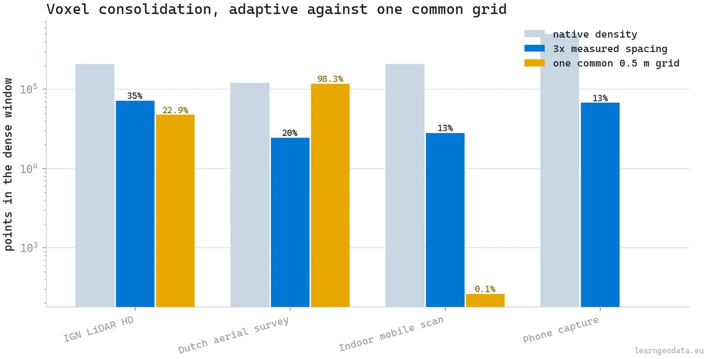
Derive the target from each capture’s own spacing instead, at 3 times the median say, and the retained fraction sits between 13.4 and 34.5 percent across all four. That is a sane reduction whichever file you point it at.
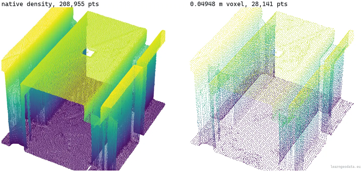
Now impose one shared 0.5 metre grid, the sort of value that lands in a YAML file and never moves. The aerial tile keeps 98.34 percent of its points, so the step did nothing. The indoor scan keeps 262 points out of 208,955.
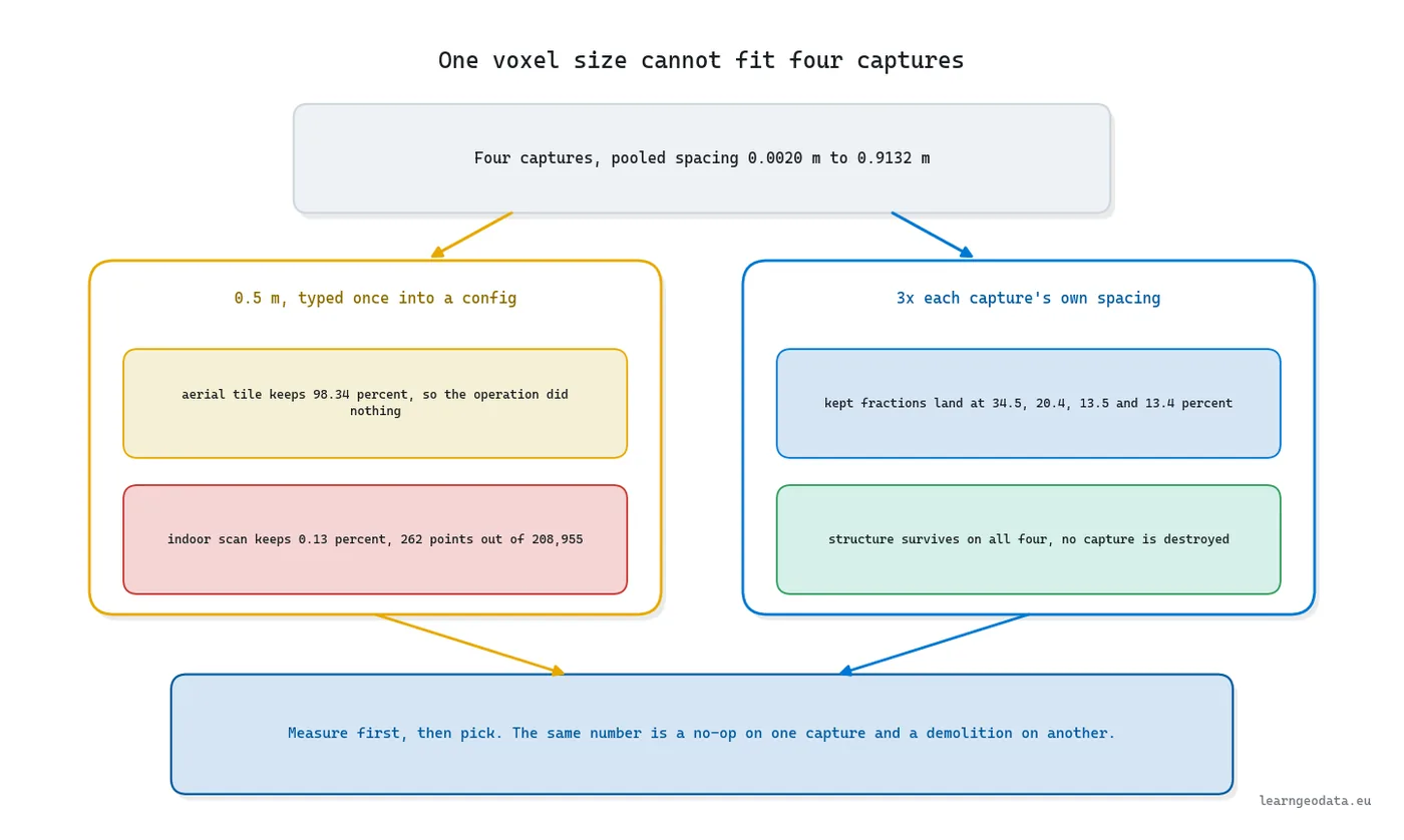
🦚 Florent’s Note: I keep coming back to that 262. Nothing crashed. The LAZ file writes, opens, renders, and passes every structural check you could throw at it, and there is no building left inside it. That is the whole reason measurement belongs before resampling instead of after, and avoiding it costs you a single KD-tree query on a window of points you were going to read anyway.
Two details decide whether your voxel step is lossless enough to trust.
First, bring the attributes along with the geometry, since bare coordinates force a nearest-neighbour rejoin that nobody schedules.
Second, choose carefully which position survives each cell. The cell centre is the worst option, because grid centres add a bias you will later see as terracing across any pitched roof. Averaging is not much better: it invents a coordinate no instrument recorded.
Compute that average anyway, then spend it. Use it only to pick the real measured point nearest to it. Every surviving row then keeps its own position, class and timestamp, all from one moment of one sensor.
The bill is around a third of a voxel of extra scatter at the ninety-fifth percentile, and it buys you a file in which every point is something that happened.
While you are emitting artefacts, emit a footprint too. A polygon of a few hundred bytes answers whether a capture covers a site without opening a point file, and a thousand of them in a spatial index give you a searchable catalogue.
Reach for the concave hull in shapely, not the convex one, because a convex boundary drawn around an L-shaped floor claims a corner the scanner never saw. Write it twice, in the survey team’s own system and in WGS84, since both consumers speak the same OGC well-known text grammar.
The area ratio between the two hulls comes free and reads like a quality score: rectangular airborne deliveries scored 0.996 and 0.998, an indoor floor 0.959, and a phone capture 0.800.
Here is the part worth stealing for whatever pipeline you write next. Shapely’s concave hull takes a dimensionless ratio, so the tempting move is to try a few and hard-code the prettiest. I picked 0.08 exactly that way.
Underneath, the library turns that ratio into a real distance anchored on the longest edge of the triangulation, which is set by the biggest hole in the capture and has nothing to do with how densely the sensor sampled.
Measured on the four files, 0.08 let a boundary leap 28 nearest-neighbour spacings on the French tile, 31 on the Dutch one, 67 indoors and 26 on the phone. One config value, four incompatible rules running in production.
Write the rule in the only unit your data defines, a permitted bridging gap of so many measured spacings, and the four ratios come out different precisely so the policy can stay the same.
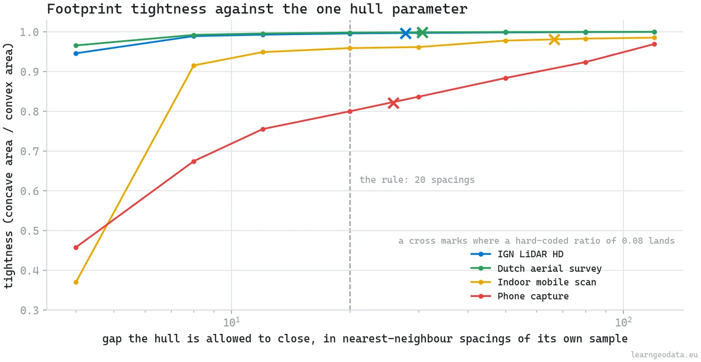
One caveat rides on that 0.800. Widen the permitted gap on the phone capture and its tightness climbs from 0.458 towards 0.969 without ever flattening, so that footprint has no natural scale to settle on. A tightness quoted without its bridging length is an opinion, not a measurement, so put both in the manifest.
Five Point Cloud Ingestion Mistakes and How to Fix Them
Five traps catch nearly everybody, and each one has a short fix.
1. Benchmarking a read. Point records load lazily, so the call returns at once and the real bill arrives when you first touch a coordinate array. Any timing you took in between is a fiction. Iterate over chunks and harvest what you need from each as it passes.
2. Leaving the write scale at a default. Serialize a millimetre-resolution scan through a header that still says 0.01 metres and you have quantized away the precision you paid a surveyor for, into a file that passes every structural check afterwards. Set the scale from the spacing you measured, around one hundredth of it, then read the file back and compare. When it is right, the largest discrepancy is exactly half the scale.
3. Leaving the offset at zero. A northing of 6,264,000 metres over a 0.001 metre scale wants more steps than a signed 32-bit integer can count to. Anchor the offset on the tile’s own corner.
4. Trusting a height transform without asking whether its grid exists. PROJ falls back to a ballpark vertical step and calls that success.
5. Inferring a coordinate system from how big the numbers look. It works until the delivery where it does not, and then costs you a reprocessing campaign and an awkward email.
🪐 System Thinking Note: The gap ledger turns out to be the commercial artefact, which nobody expects. Six gaps on one file, three on the next, then seven and ten: 26 plain sentences about what each capture cannot support. Think about how a scan-to-BIM team currently learns a delivery is unusable. A modeller spends two days on it and then complains. Slot a 60 second gate in front of that, stamping every arrival accept, query or reject, and you have changed the economics without changing anybody’s workflow.
Get ingestion right and everything above it gets easier. The processing layer sitting directly on top is the LiDAR point cloud processing guide, the grouping stage is the point cloud segmentation and clustering guide, the wider map is the 3D spatial AI with Python guide, and how these files come into existence at all is the 3D data capture and meshing guide.
Build Your Point Cloud Ingestion Layer This Week
You do not need a project to start.
Pick the archive folder you keep postponing, block out an hour, and run the header probe across everything in it. Read what your own files say about themselves, without opening one.
Then take the three or four that matter and measure their spacing on a handful of native-density windows spread across each file, never on a thinned copy. Put those numbers beside the ones your configs assume.
My guess is that one file disagrees with you sharply, and that a channel you have been trusting turns out flat. Two functions, one hour.

Want a free hands-on start? The free 3D mission puts you in front of real point clouds with the same measure-first discipline. Prefer to build the entire chain, from raw captures through to spatial systems other people depend on? That is the shape of the 3D AI Program, and more build-alongs live on the 3D Geodata Academy blog and on my Medium profile.
So here is my question back to you. When somebody asks how good your last delivery was, can you answer with a measurement, or only with an impression?
Frequently Asked Questions About Point Cloud Ingestion
What Does a Point Cloud Ingestion Layer Do?
It stands between your sensors and your code, and its only product is uniformity. Whatever container arrives, it emits the same structure: coordinates, a known set of attribute channels, a stated coordinate system and unit with a named source, a provenance trail, and a written list of everything it could not determine.
Nothing above that boundary asks which device produced the data, so adopting a new scanner becomes a small job rather than a branch in five modules. The laspy documentation covers the LAS and LAZ reading side.
Can I Open a 40 Million Point LAZ File on a Laptop?
Yes, provided you never hold it whole. Geometry alone at float64 comes to 966 MB for 40 million rows, before a single attribute.
Start with the header, which answers count, extent and coordinate system in about 1 millisecond. Then iterate the file in chunks and keep only the fraction you need. A 221.5 MB tile decimates that way in 4.6 seconds.
Should I Guess a Coordinate System When a File Does Not Declare One?
No. Coordinate magnitudes look diagnostic and are not, because national grids occupy overlapping numeric ranges and a wrong guess stays plausible for years.
Allow your layer three outcomes: read from the file, asserted by a person you can name, or unknown. 2 of the 4 captures behind this guide landed in that third category. The OGC well-known text standard covers how a declaration should look, and the ASPRS LAS specification covers where it belongs.
Is Point Count a Good Proxy for Point Cloud Density?
No, because it hides where the returns landed. Take the nearest-neighbour distance instead: sample the cloud, query two neighbours per sample, throw away the self-match, and keep the median with a percentile range around it.
Run it at native density, because a thinned copy of one airborne tile answered 0.91222 metres where the untouched data answered 0.1253 metres, wrong by a factor of 7.3. Then run it in several places, because a single central box on that same tile still came back 13 percent optimistic.
My Heights Came Back Unchanged After Reprojection. Why?
PROJ could not find the geoid grid the operation needed, so it fell back on a ballpark vertical step that hands the height straight through, and a fallback is not an error in its eyes.
Build a TransformerGroup towards EPSG:4979 and inspect what it reports: on a compound Dutch system it listed 3 usable operations, 2 blocked by an absent grid, and gave its preferred choice an accuracy of -1.0. Grids come from cdn.proj.org, as the pyproj transformation grid documentation explains.
What Should I Install to Build This?
The stack stays small. laspy with its lazrs backend handles LAS, LAZ and COPC in one dependency. pyproj covers coordinate work and the grid availability checks. shapely produces polygons and well-known text. Open3D covers inspection and general geometry. NumPy underpins all of them and SciPy adds the KD-tree.

