3D Reconstruction Pipeline: Photo to Model Workflow Guide

The 3D Reconstruction pipeline, to get from 2D photographs to 3D models follows a structured path. 

This path consists of distinct steps that build upon each other to transform flat images into spatial information. 

Understanding this pipeline is crucial for anyone looking to create high-quality 3D reconstructions.

Let me explain…

Most people think 3D reconstruction means:

• Taking random photos around an object
• Pressing a button in expensive software
• Waiting for magic to happen
• Getting perfect results every time
• Skipping the fundamentals

No thanks.

The most impactful 3D Reconstruction pipeline I have seen are tied to careful understanding of the core components.

They are based on fewer images but are positioned better. Also, innovators spend less time processing but achieve cleaner results. Finally, we can troubleshoot faster because we know exactly where to look.

Therefore, this hints at a nice lesson:

Your 3D models can only be as good as your understanding of how they’re created.

Looking at this from a scientific perspective is really key.

Let us dive right into it!

🦊 Florent: If you are new to my (3D) writing world, welcome! We are going on an exciting adventure that will allow you to master an essential 3D Python skill.

Once the scene is laid out, we embark on the Python journey. Everything is provided, included resources at the end. You will see Tips (🦚Notes and 🌱Growing) to help you get the most out of this article. Thanks to the 3D Geodata Academy for supporting the endeavor. This article is inspired by a small section of Module 1 of the 3D Reconstructor OS Course.

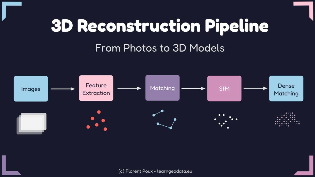
The Complete 3D Reconstruction Pipeline

Let me highlight the 3D Reconstruction pipeline with Photogrammetry. The process follows a logical sequence of steps, as illustrated below.

What is important to note, is that each step builds upon the previous one. Therefore, the quality of each stage directly impacts the final result, which is very important to have in mind!

🦊 Florent: Understanding the entire process is crucial for troubleshooting workflows due to its sequential nature.

With that in mind, let’s detail each step, focusing on both the theory and practical implementation.

Natural Feature Extraction: Finding the Distinctive Points

Natural feature extraction is the foundation of the photogrammetry process. It identifies distinctive points in images that can be reliably located across multiple photographs.

These points serve as anchors that tie different views together in the 3D Reconstruction pipeline

🌱 Florent’s Note: When working with low-texture objects, consider adding temporary markers or texture patterns to improve feature extraction results.

Common feature extraction algorithms include:

Algorithm	Strengths	Weaknesses	Best For
SIFT	Scale and rotation invariant	Computationally expensive	High-quality, general-purpose reconstruction
SURF	Faster than SIFT	Less accurate than SIFT	Quick prototyping
ORB	Very fast, no patent restrictions	Less robust to viewpoint changes	Real-time applications

Let’s implement a simple feature extraction using OpenCV:

#%% SECTION 1: Natural Feature Extraction
import cv2
import numpy as np
import matplotlib.pyplot as plt
def extract_features(image_path, feature_method='sift', max_features=2000):
    """
    Extract features from an image using different methods.
    """
    # Read the image in color and convert to grayscale
    img = cv2.imread(image_path)
    if img is None:
        raise ValueError(f"Could not read image at {image_path}")
    
    gray = cv2.cvtColor(img, cv2.COLOR_BGR2GRAY)
    
    # Initialize feature detector based on method
    if feature_method.lower() == 'sift':
        detector = cv2.SIFT_create(nfeatures=max_features)
    elif feature_method.lower() == 'surf':
        # Note: SURF is patented and may not be available in all OpenCV distributions
        detector = cv2.xfeatures2d.SURF_create(400)  # Adjust threshold as needed
    elif feature_method.lower() == 'orb':
        detector = cv2.ORB_create(nfeatures=max_features)
    else:
        raise ValueError(f"Unsupported feature method: {feature_method}")
    
    # Detect and compute keypoints and descriptors
    keypoints, descriptors = detector.detectAndCompute(gray, None)
    
    # Create visualization
    img_with_features = cv2.drawKeypoints(
        img, keypoints, None, 
        flags=cv2.DRAW_MATCHES_FLAGS_DRAW_RICH_KEYPOINTS
    )
    
    print(f"Extracted {len(keypoints)} {feature_method.upper()} features")
    
    return keypoints, descriptors, img_with_features
image_path = "sample_image.jpg"  # Replace with your image path
# Extract features with different methods
kp_sift, desc_sift, vis_sift = extract_features(image_path, 'sift')
kp_orb, desc_orb, vis_orb = extract_features(image_path, 'orb')

What I do here is run through an image, and hunt for distinctive patterns that stand out from their surroundings.

These patterns create mathematical “signatures” called descriptors that remain recognizable even when viewed from different angles or distances. 

Think of them as unique fingerprints that can be matched across multiple photographs.

The visualization step reveals exactly what the algorithm finds important in your image.

# Display results
plt.figure(figsize=(12, 6))
    
plt.subplot(1, 2, 1)
plt.title(f'SIFT Features ({len(kp_sift)})')
plt.imshow(cv2.cvtColor(vis_sift, cv2.COLOR_BGR2RGB))
plt.axis('off')
    
plt.subplot(1, 2, 2)
plt.title(f'ORB Features ({len(kp_orb)})')
plt.imshow(cv2.cvtColor(vis_orb, cv2.COLOR_BGR2RGB))
plt.axis('off')
    
plt.tight_layout()
plt.show()

Notice how corners, edges, and textured areas attract more keypoints, while smooth or uniform regions remain largely ignored.

This visual feedback is invaluable for understanding why some objects reconstruct better than others.

🦥 Geeky Note: The max_features parameter is critical. Setting it too high can dramatically slow processing and capture noise, while setting it too low might miss important details. For most objects, 2000-5000 features provide a good balance, but I’ll push it to 10,000+ for highly detailed architectural reconstructions.

Feature Matching: Connecting Images Together

Once features are extracted, the next step is to find correspondences between images. This process identifies which points in different images represent the same physical point in the real world. Feature matching creates the connections needed to determine camera positions.

I’ve seen countless attempts fail because the algorithm couldn’t reliably connect the same points across different images.

The ratio test is the silent hero that weeds out ambiguous matches before they poison your reconstruction.

#%% SECTION 2: Feature Matching
import cv2
import numpy as np
import matplotlib.pyplot as plt
def match_features(descriptors1, descriptors2, method='flann', ratio_thresh=0.75):
    """
    Match features between two images using different methods.
    """
    # Convert descriptors to appropriate type if needed
    if descriptors1 is None or descriptors2 is None:
        return []
    
    if method.lower() == 'flann':
        # FLANN parameters
        if descriptors1.dtype != np.float32:
            descriptors1 = np.float32(descriptors1)
        if descriptors2.dtype != np.float32:
            descriptors2 = np.float32(descriptors2)
            
        FLANN_INDEX_KDTREE = 1
        index_params = dict(algorithm=FLANN_INDEX_KDTREE, trees=5)
        search_params = dict(checks=50)  # Higher values = more accurate but slower
        
        flann = cv2.FlannBasedMatcher(index_params, search_params)
        matches = flann.knnMatch(descriptors1, descriptors2, k=2)
    else:  # Brute Force
        # For ORB descriptors
        if descriptors1.dtype == np.uint8:
            bf = cv2.BFMatcher(cv2.NORM_HAMMING, crossCheck=False)
        else:  # For SIFT and SURF descriptors
            bf = cv2.BFMatcher(cv2.NORM_L2, crossCheck=False)
        
        matches = bf.knnMatch(descriptors1, descriptors2, k=2)
    
    # Apply Lowe's ratio test
    good_matches = []
    for match in matches:
        if len(match) == 2:  # Sometimes fewer than 2 matches are returned
            m, n = match
            if m.distance < ratio_thresh * n.distance:
                good_matches.append(m)
    
    return good_matches
def visualize_matches(img1, kp1, img2, kp2, matches, max_display=100):
    """
    Create a visualization of feature matches between two images.
    """
    # Limit the number of matches to display
    matches_to_draw = matches[:min(max_display, len(matches))]
    
    # Create match visualization
    match_img = cv2.drawMatches(
        img1, kp1, img2, kp2, matches_to_draw, None,
        flags=cv2.DrawMatchesFlags_NOT_DRAW_SINGLE_POINTS
    )
    
    return match_img
# Load two images
img1_path = "image1.jpg"  # Replace with your image paths
img2_path = "image2.jpg"
    
# Extract features using SIFT (or your preferred method)
kp1, desc1, _ = extract_features(img1_path, 'sift')
kp2, desc2, _ = extract_features(img2_path, 'sift')
    
# Match features
good_matches = match_features(desc1, desc2, method='flann')
    
print(f"Found {len(good_matches)} good matches")

The matching process works by comparing feature descriptors between two images, measuring their mathematical similarity. For each feature in the first image, we find its two closest matches in the second image and assess their relative distances. 

If the closest match is significantly better than the second-best (as controlled by the ratio threshold), we consider it reliable.

# Visualize matches
img1 = cv2.imread(img1_path)
img2 = cv2.imread(img2_path)
match_visualization = visualize_matches(img1, kp1, img2, kp2, good_matches)
    
plt.figure(figsize=(12, 8))
plt.imshow(cv2.cvtColor(match_visualization, cv2.COLOR_BGR2RGB))
plt.title(f"Feature Matches: {len(good_matches)}")
plt.axis('off')
plt.tight_layout()
plt.show()

Visualizing these matches reveals the spatial relationships between your images.

Good matches form a consistent pattern that reflects the transform between viewpoints, while outliers appear as random connections. 

This pattern provides immediate feedback on image quality and camera positioning—clustered, consistent matches suggest good reconstruction potential.

🦥 Geeky Note: The ratio_thresh parameter (0.75) is Lowe’s original recommendation and works well in most situations. Lower values (0.6-0.7) produce fewer but more reliable matches, which is preferable for scenes with repetitive patterns. Higher values (0.8-0.9) yield more matches but increase the risk of outliers contaminating your reconstruction.

Beautiful, now, let us move at the main stage of the 3D Reconstruction pipeline: the Structure from Motion node.

Structure From Motion of 3D Reconstruction Pipeline

Structure from Motion (SfM) reconstructs both the 3D scene structure and camera motion from the 2D image correspondences. This process determines where each photo was taken from and creates an initial sparse point cloud of the scene.

Key steps in SfM include:

1. Estimating the fundamental or essential matrix between image pairs
2. Recovering camera poses (position and orientation)
3. Triangulating 3D points from 2D correspondences
4. Building a track graph to connect observations across multiple images

The essential matrix encodes the geometric relationship between two camera viewpoints, revealing how they’re positioned relative to each other in space.

This mathematical relationship is the foundation for reconstructing both the camera positions and the 3D structure they observed.

#%% SECTION 3: Structure from Motion
import cv2
import numpy as np
import matplotlib.pyplot as plt
from mpl_toolkits.mplot3d import Axes3D
def estimate_pose(kp1, kp2, matches, K, method=cv2.RANSAC, prob=0.999, threshold=1.0):
    """
    Estimate the relative pose between two cameras using matched features.
    """
    # Extract matched points
    pts1 = np.float32([kp1[m.queryIdx].pt for m in matches])
    pts2 = np.float32([kp2[m.trainIdx].pt for m in matches])
    
    # Estimate essential matrix
    E, mask = cv2.findEssentialMat(pts1, pts2, K, method, prob, threshold)
    
    # Recover pose from essential matrix
    _, R, t, mask = cv2.recoverPose(E, pts1, pts2, K, mask=mask)
    
    inlier_matches = [matches[i] for i in range(len(matches)) if mask[i] > 0]
    print(f"Estimated pose with {np.sum(mask)} inliers out of {len(matches)} matches")
    
    return R, t, mask, inlier_matches
def triangulate_points(kp1, kp2, matches, K, R1, t1, R2, t2):
    """
    Triangulate 3D points from two views.
    """
    # Extract matched points
    pts1 = np.float32([kp1[m.queryIdx].pt for m in matches])
    pts2 = np.float32([kp2[m.trainIdx].pt for m in matches])
    
    # Create projection matrices
    P1 = np.dot(K, np.hstack((R1, t1)))
    P2 = np.dot(K, np.hstack((R2, t2)))
    
    # Triangulate points
    points_4d = cv2.triangulatePoints(P1, P2, pts1.T, pts2.T)
    
    # Convert to 3D points
    points_3d = points_4d[:3] / points_4d[3]
    
    return points_3d.T
def visualize_points_and_cameras(points_3d, R1, t1, R2, t2):
    """
    Visualize 3D points and camera positions.
    """
    fig = plt.figure(figsize=(10, 8))
    ax = fig.add_subplot(111, projection='3d')
    
    # Plot points
    ax.scatter(points_3d[:, 0], points_3d[:, 1], points_3d[:, 2], c='b', s=1)
    
    # Helper function to create camera visualization
    def plot_camera(R, t, color):
        # Camera center
        center = -R.T @ t
        ax.scatter(center[0], center[1], center[2], c=color, s=100, marker='o')
        
        # Camera axes (showing orientation)
        axes_length = 0.5  # Scale to make it visible
        for i, c in zip(range(3), ['r', 'g', 'b']):
            axis = R.T[:, i] * axes_length
            ax.quiver(center[0], center[1], center[2], 
                      axis[0], axis[1], axis[2], 
                      color=c, arrow_length_ratio=0.1)
    
    # Plot cameras
    plot_camera(R1, t1, 'red')
    plot_camera(R2, t2, 'green')
    
    ax.set_title('3D Reconstruction: Points and Cameras')
    ax.set_xlabel('X')
    ax.set_ylabel('Y')
    ax.set_zlabel('Z')
    
    # Try to make axes equal
    max_range = np.max([
        np.max(points_3d[:, 0]) - np.min(points_3d[:, 0]),
        np.max(points_3d[:, 1]) - np.min(points_3d[:, 1]),
        np.max(points_3d[:, 2]) - np.min(points_3d[:, 2])
    ])
    
    mid_x = (np.max(points_3d[:, 0]) + np.min(points_3d[:, 0])) * 0.5
    mid_y = (np.max(points_3d[:, 1]) + np.min(points_3d[:, 1])) * 0.5
    mid_z = (np.max(points_3d[:, 2]) + np.min(points_3d[:, 2])) * 0.5
    
    ax.set_xlim(mid_x - max_range * 0.5, mid_x + max_range * 0.5)
    ax.set_ylim(mid_y - max_range * 0.5, mid_y + max_range * 0.5)
    ax.set_zlim(mid_z - max_range * 0.5, mid_z + max_range * 0.5)
    
    plt.tight_layout()
    plt.show()

🦥 Geeky Note: The RANSAC threshold parameter (threshold=1.0) determines how strict we are about geometric consistency. I’ve found that 0.5-1.0 works well for controlled environments, but increasing to 1.5-2.0 helps with outdoor scenes where wind might cause slight camera movements. The probability parameter (prob=0.999) ensures high confidence but increases computation time; 0.95 is sufficient for prototyping.

The essential matrix estimation uses matched feature points and the camera’s internal parameters to calculate the geometric relationship between images.

This relationship is then decomposed to extract rotation and translation information – essentially determining where each photo was taken from in 3D space. The accuracy of this step directly affects everything that follows.

# This is a simplified example - in practice you would use images and matches
# from the previous steps
    
# Example camera intrinsic matrix (replace with your calibrated values)
K = np.array([
        [1000, 0, 320],
        [0, 1000, 240],
        [0, 0, 1]
])
    
# For first camera, we use identity rotation and zero translation
R1 = np.eye(3)
t1 = np.zeros((3, 1))
    
# Load images, extract features, and match as in previous sections
img1_path = "image1.jpg"  # Replace with your image paths
img2_path = "image2.jpg"
    
img1 = cv2.imread(img1_path)
img2 = cv2.imread(img2_path)
    
kp1, desc1, _ = extract_features(img1_path, 'sift')
kp2, desc2, _ = extract_features(img2_path, 'sift')
    
matches = match_features(desc1, desc2, method='flann')
    
# Estimate pose of second camera relative to first
R2, t2, mask, inliers = estimate_pose(kp1, kp2, matches, K)
    
# Triangulate points
points_3d = triangulate_points(kp1, kp2, inliers, K, R1, t1, R2, t2)

Once camera positions are established, triangulation projects rays from matched points in multiple images to determine where they intersect in 3D space.

# Visualize the result
visualize_points_and_cameras(points_3d, R1, t1, R2, t2)

These intersections form the initial sparse point cloud, providing the skeleton upon which dense reconstruction will later build. The visualization shows both the reconstructed points and the camera positions, helping you understand the spatial relationships in your dataset.

🌱 Florent’s Note: SfM works best with a good network of overlapping images. Aim for at least 60% overlap between adjacent images for reliable reconstruction.

Bundle Adjustment: Optimizing for Accuracy

There is an extra optimization stage that comes in within the Structure from Motion “compute node”. 

This is called: Bundle adjustment.

It is a refinement step that jointly optimizes camera parameters and 3D point positions. What that means, is that it minimizes the reprojection error, i.e. the difference between observed image points and the projection of their corresponding 3D points.

Does this make sense to you? Essentially, this optimization is great as it permits to:

• improves the accuracy of the reconstruction
• correct for accumulated drift
• Ensures global consistency of the model

At this stage, this should be enough to get a good intuition of how it works.

🌱 Florent’s Note: In larger projects, incremental bundle adjustment (optimizing after adding each new camera) can improve both speed and stability compared to global adjustment at the end.

Dense Matching: Creating Detailed Reconstructions

After establishing camera positions and sparse points, the final step is dense matching to create a detailed representation of the scene. 

Dense matching uses the known camera parameters to match many more points between images, resulting in a complete point cloud.

Common approaches include:

• Multi-View Stereo (MVS)
• Patch-based Multi-View Stereo (PMVS)
• Semi-Global Matching (SGM)

Putting It All Together: Practical Tools

The theoretical pipeline is implemented in several open-source and commercial software packages. Each offers different features and capabilities:

Tool	Strengths	Use Case	Pricing
COLMAP	Highly accurate, customizable	Research, precise reconstructions	Free, open-source
OpenMVG	Modular, extensive documentation	Education, integration with custom pipelines	Free, open-source
Meshroom	User-friendly, node-based interface	Artists, beginners	Free, open-source
RealityCapture	Extremely fast, high-quality results	Professional, large-scale projects	Commercial

These tools package the various pipeline steps described above into a more user-friendly interface, but understanding the underlying processes is still essential for troubleshooting and optimization.

Automating the reconstruction pipeline saves countless hours of manual work.

The real productivity boost comes from scripting the entire process end-to-end, from raw photos to dense point cloud.

COLMAP’s command-line interface makes this automation possible, even for complex reconstruction tasks.

🌱 Florent’s Note: You can find the complete automated pipeline with COLMAP in the 3D Reconstructor OS, Module 1.

The script orchestrates a series of COLMAP operations that would normally require manual intervention at each stage. It handles the progression from feature extraction through matching, sparse reconstruction, and finally dense reconstruction – maintaining the correct data flow between steps. This automation becomes invaluable when processing multiple datasets or when iteratively refining reconstruction parameters.

One key aspect is the automatic selection of the largest reconstructed model. In challenging datasets, COLMAP sometimes creates multiple disconnected reconstructions rather than a single cohesive model. 

The script intelligently identifies and continues with the most complete reconstruction, using image count as a proxy for model quality and completeness.

🦥 Geeky Note: The –SiftExtraction.use_gpu and –SiftMatching.use_gpu flags enable GPU acceleration, speeding up processing by 5-10x. For dense reconstruction, the –PatchMatchStereo.geom_consistency true parameter significantly improves quality by enforcing consistency across multiple views, at the cost of longer processing time.

The Power of Understanding the Pipeline

Understanding the full reconstruction pipeline gives you control over your 3D modeling process. When you encounter issues, knowing which stage might be causing problems allows you to target your troubleshooting efforts effectively.

As illustrated, common issues and their sources include:

1. Missing or incorrect camera poses: Feature extraction and matching problems
2. Incomplete reconstruction: Insufficient image overlap
3. Noisy point clouds: Poor bundle adjustment or camera calibration
4. Failed reconstruction: Problematic images (motion blur, poor lighting)

The ability to diagnose these issues comes from a deep understanding of how each pipeline component works and interacts with others.

Next Steps: Practice and Automation

Now that you understand the pipeline, it’s time to put it into practice. Experiment with the provided code examples and try automating the process for your own datasets.

Start with small, well-controlled scenes and gradually tackle more complex environments as you gain confidence.

Remember that the quality of your input images dramatically affects the final result. Take time to capture high-quality photographs with good overlap, consistent lighting, and minimal motion blur.

🌱 Florent ‘s Note:  Consider starting a small personal project to reconstruct an object you own. Document your process, including the issues you encounter and how you solve them – this practical experience is invaluable.

If you want to build proper expertise, consider
the 3D Reconstructor OS Course ▶️,
or 3D Data Science with Python 📕 (O’Reilly)

References and useful resources

I compiled for you some interesting software, tools, and useful algorithm extended documentation:

Software and Tools

• COLMAP – Free, open-source 3D reconstruction software
• OpenMVG – Open Multiple View Geometry library
• Meshroom – Free node-based photogrammetry software
• RealityCapture – Commercial high-performance photogrammetry software
• Agisoft Metashape – Commercial photogrammetry and 3D modeling software
• OpenCV – Computer vision library with feature detection implementations
• 3DF Zephyr – Photogrammetry software for 3D reconstruction
• Python – Programming language ideal for 3D reconstruction automation

Algorithms

• SIFT (Scale-Invariant Feature Transform) – Robust feature detection algorithm
• SURF (Speeded-Up Robust Features) – Fast feature detection algorithm
• ORB (Oriented FAST and Rotated BRIEF) – Efficient alternative to SIFT and SURF
• RANSAC (Random Sample Consensus) – Used for outlier rejection in matching
• Structure from Motion (SfM) – Algorithm for recovering 3D structure from 2D images
• Multi-View Stereo (MVS) – Dense reconstruction algorithm
• Bundle Adjustment – Optimization technique for camera poses and 3D points
• FLANN (Fast Library for Approximate Nearest Neighbors) – Fast matching algorithm for feature descriptors

About the author

Florent Poux, Ph.D. is a Scientific and Course Director focused on educating engineers on leveraging AI and 3D Data Science. He leads research teams and teaches 3D Computer Vision at various universities. His current aim is to ensure humans are correctly equipped with the knowledge and skills to tackle 3D challenges for impactful innovations.

Resources

1. 🏆Awards: Jack Dangermond Award
2. 📕Book: 3D Data Science with Python
3. 📜Research: 3D Smart Point Cloud (Thesis)
4. 🎓Courses: 3D Geodata Academy Catalog
5. 💻Code: Florent’s Github Repository
6. 💌3D Tech Digest: Weekly Newsletter