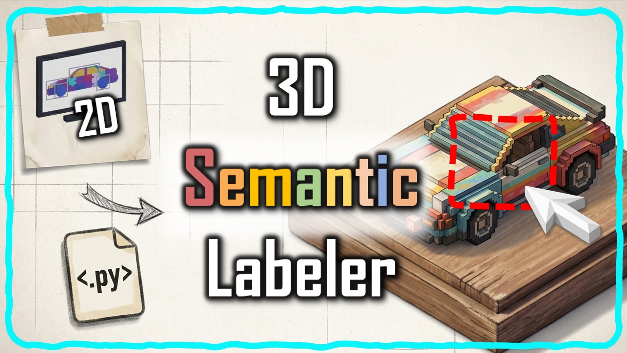
This article walks through a complete 3D point cloud labeling pipeline built in Python. You paint semantic masks on ordinary phone photos, and the system projects those labels into a fully annotated 3D scene using camera geometry and spatial indexing. No GPU, no neural network training, no manual point-by-point clicking.
What you’ll learn in this article:
- How to turn 5 painted photos into 800,000 labeled 3D points in under 5 minutes
- The 6-step Python pipeline for 3D point cloud labeling from photographs
- Why pinhole back-projection and KD-tree fusion are the key architectural decisions
- How to export labeled scenes as GLB/PLY for downstream analysis
- Why understanding this architecture matters more than the code itself
Estimated reading time: 13 minutes
AI writes Python code now, but here’s what that actually changes for 3D point cloud labeling
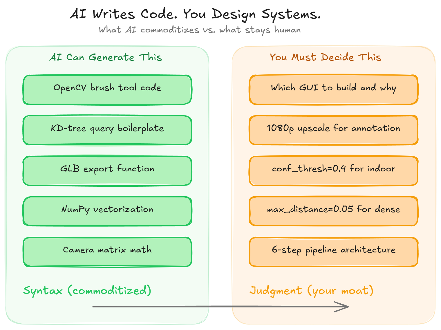
Any large language model can generate an OpenCV brush tool in thirty seconds. You type “write me a painting GUI in Python,” and you get a working script with mouse callbacks, color pickers, and keyboard shortcuts.
It’s impressive. I won’t pretend otherwise.
But here’s the thing: syntax was never the hard part. The hard part is knowing you need a painting GUI in the first place, that it should upscale to 1080p for comfortable annotation, that five semantic classes are enough for most indoor scenes, and that the mask it produces has to feed a pinhole back-projection step that converts your 2D brush strokes into 3D labeled coordinates.
That chain of decisions is architecture. No code generator can assemble it from a single prompt.
🦚 Florent’s Note: I’ve spent the last decade building 3D point cloud labeling pipelines for warehouse robotics, construction inspection, and spatial analysis. And the pattern I keep seeing is always the same. The people who understand the full workflow ship working tools. The people who only know how to prompt for code? They get stuck the moment two components need to talk to each other.
So what does this article actually give you? It walks through the architecture behind a Python tool for 3D point cloud labeling that turns phone photos into fully labeled 3D scenes. And it explains why understanding that architecture is the skill that’ll matter most in spatial AI over the next five years.
How to label 800,000 3D points without clicking through them one by one
You took twenty photos of an object with your phone and ran them through a monocular depth estimator like Depth-Anything-3. A dense, colorful 3D point cloud came out in minutes. The geometry’s accurate, the colors are vivid, the reconstruction covers every visible surface.
But this point cloud has no idea what anything is.
Every point carries x, y, z, and RGB, but zero semantic information. You can’t select “roof” or measure the surface area of “floor” or export only the “furniture” class for downstream analysis. And honestly, labeling 800,000 points by hand in a 3D viewer isn’t realistic for anyone.
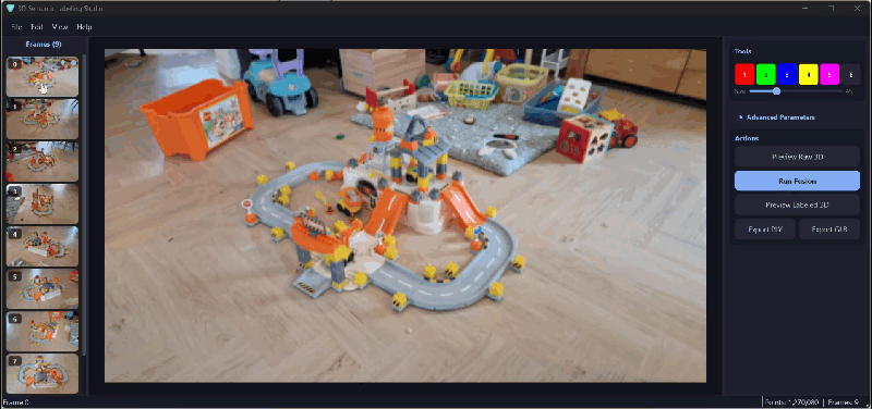
🦥 Geeky Note: The KIDS dataset I use here has 847,392 points across 15 frames at 518×518 resolution. The NPZ archive is about 150 MB. For scenes above 5 million points, you’ll want to reduce the batch_size in the fusion step from 100,000 to 50,000 to keep memory bounded.
So what do you do? You stop thinking in 3D and start thinking in 2D. It’s like trying to organize a messy warehouse: you don’t rearrange every box individually, you take a photo from a few angles, draw regions on the photos, and let the map do the rest.
Same principle here. Humans are fast annotators on flat images. A broad brush stroke on a photograph covers thousands of 3D points after projection, and the camera geometry transfers those labels automatically.
You paint on five photos. The algorithm handles the rest.
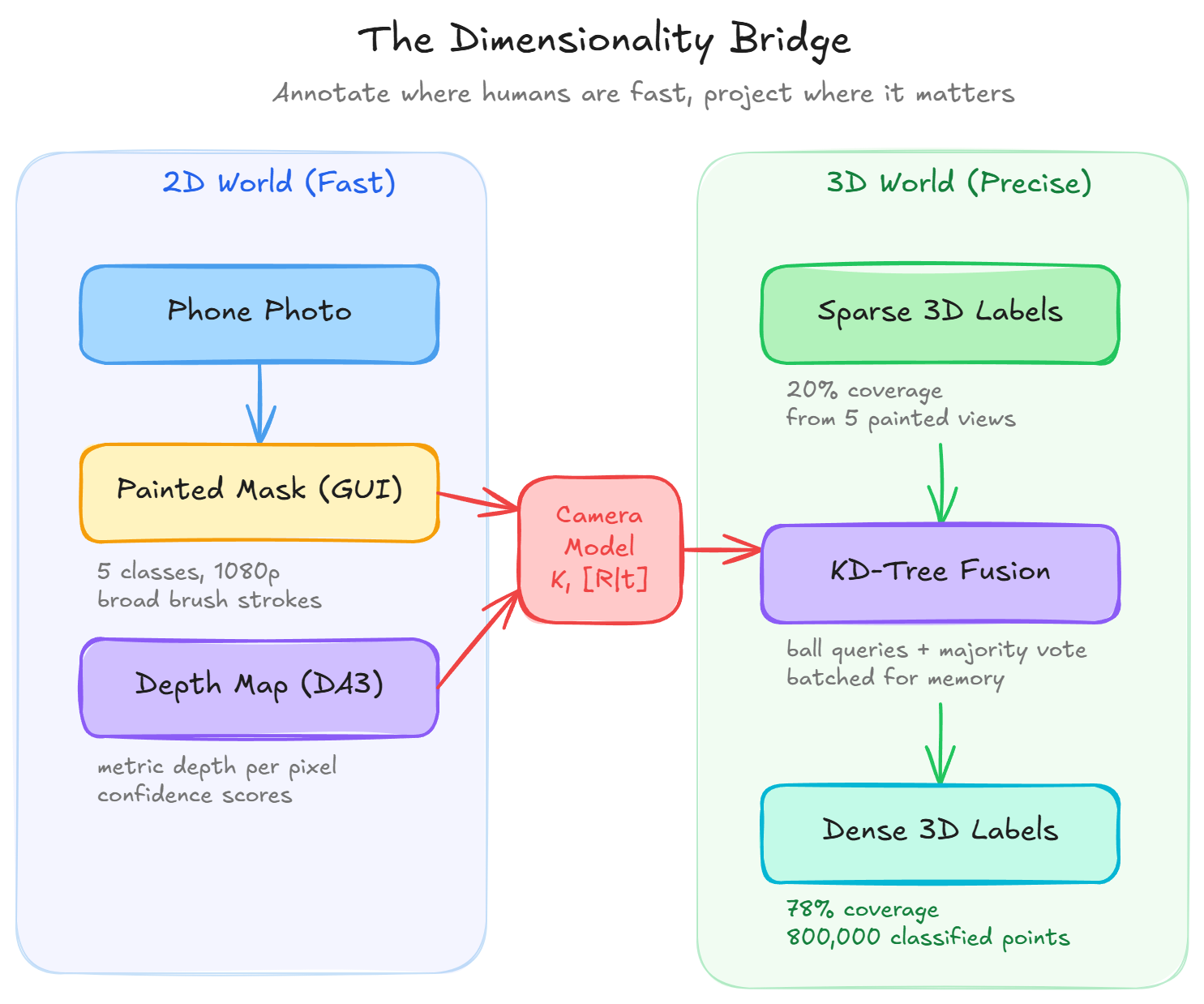
🪐 System Thinking Note: This is what I call dimensionality bridging. You exploit the dimension where the task is easiest (2D for annotation), then project the result where it’s needed (3D for analysis). Every time you see a 2D-to-3D or 3D-to-2D pipeline in computer vision, the same principle applies. Understanding this pattern lets you design new pipelines for problems nobody’s solved yet.
Python setup for 3D point cloud labeling: install the toolkit in one command
The entire pipeline runs on Python 3.9 to 3.13 with no GPU required, because the heavy depth inference already happened upstream in Depth-Anything-3. One command gets you everything:
pip install numpy open3d matplotlib scipy opencv-python trimeshVerify your setup:
import numpy as np
import open3d as o3d
import cv2
import matplotlib.pyplot as plt
from scipy.spatial import cKDTree
print("All imports OK")
🦥 Geeky Note: Windows, macOS, and Linux all work. The only display requirement is Step 2, where OpenCV opens a painting window. If you’re on a headless server or WSL2, you’ll need an X server (VcXsrv on Windows, or WSLg on Windows 11). On Apple Silicon, install Open3D with pip install open3d --no-cache-dir or via conda.
The dataset I use here is called KIDS: fifteen photographs of a colorful toy assembly taken with a smartphone. The previous tutorial processed these through Depth-Anything-3 and saved everything into a single reconstruction_data.npz archive.
You can also use your own photos. Anything you can walk around and snap 10-20 overlapping shots of works.
🌱 Growing Note: If you want to start from scratch with your own images (not the KIDS dataset), check the 3D reconstruction tutorial first. It covers the full Depth-Anything-3 pipeline that produces the NPZ file this tutorial consumes.
The 6-step Python pipeline for 3D point cloud labeling from photographs
The complete pipeline chains six operations where each step feeds the next:
- Load the reconstruction data from an NPZ archive
- Paint HD semantic masks on selected images through the interactive GUI
- Project each mask to 3D using pinhole back-projection with the camera intrinsics and extrinsics
- Assign labels to the full scene via nearest-neighbor matching in a cKDTree
- Fuse and propagate those labels with batched ball queries and majority voting
- Export the result as a labeled GLB with camera frustums baked in
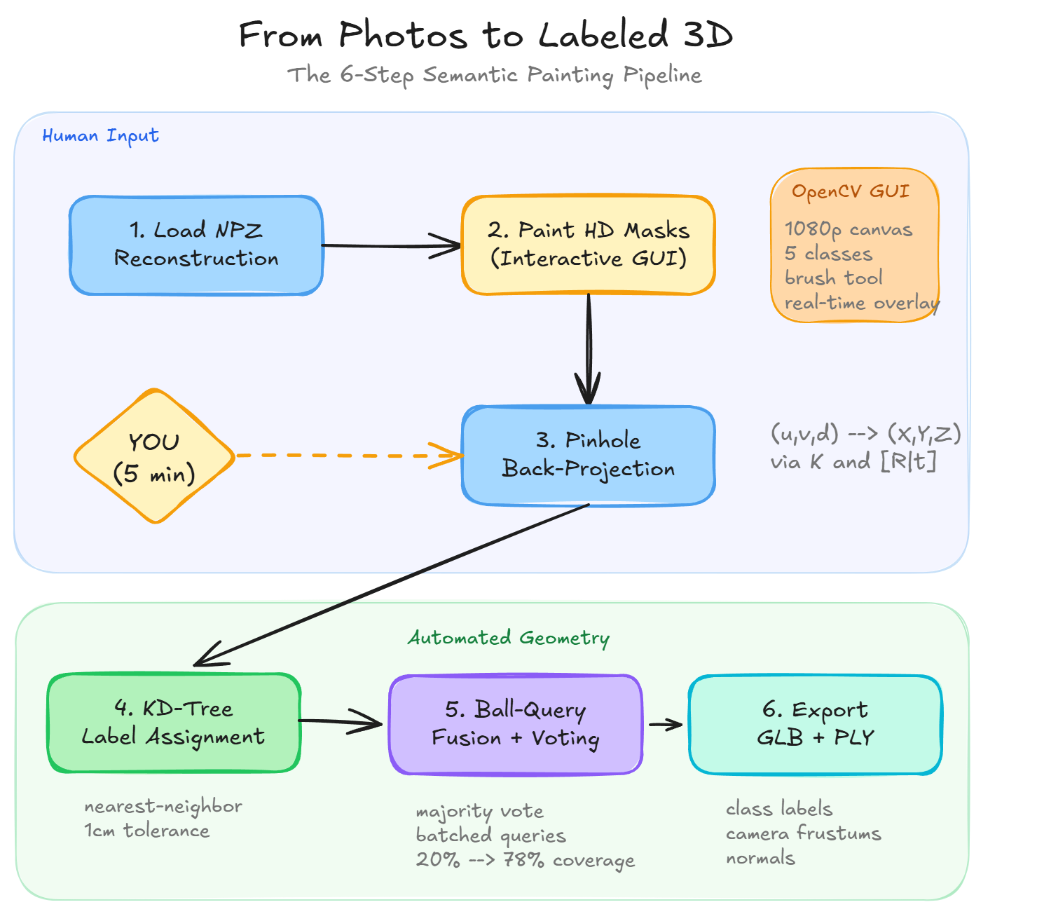
Look, the GUI sits at step two, and it’s the only moment in the entire pipeline where a human touches the data. Everything before it is automated loading. Everything after it is automated geometry.
That single interaction point is where your judgment lives.
Which surfaces to paint, how many viewpoints to cover, how aggressively to annotate. Those decisions determine the quality of the final output more than any parameter in the code.
🦚 Florent’s Note: I’ve seen teams spend days tuning the fusion algorithm when the real problem was that they only painted two viewpoints. Coverage beats precision in this pipeline. Five broad strokes across different classes from five angles beats careful pixel-level painting on one image every time.
How the interactive GUI solves the 3D point cloud labeling bottleneck
The painting GUI is an OpenCV window that upscales your image to 1080p for comfortable annotation. You switch between five semantic classes with keyboard shortcuts, and every brush stroke gets recorded into an integer mask array where each pixel holds a class ID.
Why 1080p? Because a single broad stroke at that resolution covers thousands of 3D points after projection. The upscale gives you room to paint fine details on small components without squinting at a 518×518 thumbnail.
🦥 Geeky Note: num_classes=5 isn’t a hard limit. The colormap supports 0-5 (six entries). For the KIDS toy assembly I used: base plate, walls, roof, figures, accessories. Need more? Extend the colormap arrays in both the painting module and visualization functions. I’ve gone up to 12 classes on industrial pipe racks without any performance issues.
After painting, a three-panel triptych shows you the original image, the mask classes with a tab10 colormap, and a semi-transparent overlay so you can check spatial alignment before committing to 3D projection.
Wait, that’s not quite right. The triptych isn’t just a visual check. It’s your last line of defense before the geometry pipeline takes over. If something looks off here, you catch it in seconds. If you skip this step and find out after fusion that your labels are misaligned, you’ll have to repaint and rerun everything.
🌱 Growing Note: The painting module ships with the toolkit materials available from learngeodata.eu. It contains two functions: paint_mask_hd for single-image painting and mask_multiple_images_hd for batch painting across frames. Start with single-image to get comfortable, then batch.
How pinhole back-projection converts 2D brush strokes to 3D labeled coordinates
This is where geometry takes over. Each labeled pixel from your painted mask becomes a labeled 3D point through pinhole back-projection: the inverse of how cameras form images. Instead of projecting 3D points onto a 2D sensor, you reverse the process.
Given a pixel at (u, v) with metric depth d from Depth-Anything-3, the camera intrinsics K give you the focal lengths and principal point, and the extrinsics [R|t] give you the rotation and translation to world coordinates.
The entire projection is vectorized through NumPy, which means all pixels are processed in a single pass with no Python loops.
🦥 Geeky Note: The confidence threshold conf_thresh is the most important parameter in this step. At 0.4, you get more labeled 3D points but some land in wrong locations due to depth errors. At 0.8, fewer points but higher accuracy. For the KIDS toy assembly, 0.4 works well because the texture is good and depth is reliable. For outdoor scenes with sky and glass, bump it to 0.6-0.7.
🦚 Florent’s Note: I can’t stress this enough: check your projected points visually before moving to fusion. I’ve seen projects where a team spent days tuning the fusion algorithm when the real problem was projecting garbage depth values into 3D. If the single-frame projection looks noisy, multi-frame fusion can’t fix it. The garbage-in-garbage-out principle has never been more literal than with depth-based 3D projection.
How KD-tree fusion propagates sparse labels across 800,000 3D points
One painted frame typically covers only 20-30% of the scene. To get full coverage, you paint several frames from different viewpoints and merge the labels using scipy’s cKDTree.
For each frame’s projected 3D points, the algorithm finds the closest point in the full scene and transfers the label, but only if the distance is below 0.01 meters (one centimeter). That tight tolerance prevents misassignment when depth has small errors.
Then comes the fusion step: for every unlabeled point, the algorithm looks at labeled points in its spatial neighborhood, counts the votes for each class, and assigns the majority winner. No neural network, no training. Pure spatial proximity and democratic voting.
🪐 System Thinking Note: Building the KD-tree once over the full scene (not per-frame) is the right design. Tree construction is O(N log N), each query O(log N). With 5 frames and 50k labeled points per frame, you do 250k queries against one tree instead of rebuilding 5 times. This is the kind of architectural decision that AI won’t suggest unless you know to ask for it.
🌱 Growing Note: The three parameters to tune: max_distance=0.05 (propagation radius, 5 cm for dense indoor objects, 0.15 for sparse outdoor). min_neighbors=3 (minimum votes to propagate, increase to 5-10 for noisy data). batch_size=100000 (safe for 16 GB RAM, drop to 50000 under memory pressure). These three numbers determine the quality-speed-memory tradeoff for your specific scene. The 3D Geodata Academy courses go deep on tuning these for different scan types.

What this 3D point cloud labeling toolkit gives you
- An interactive OpenCV brush tool that paints semantic masks on photographs at 1080p resolution with real-time overlay feedback
- Pinhole back-projection that converts every labeled pixel into a 3D world coordinate using depth maps from Depth-Anything-3
- KD-tree nearest-neighbor matching that transfers labels from projected points to the full scene within one-centimeter tolerance
- Batched ball-query fusion with majority voting that propagates sparse annotations into dense scene-wide labels
- GLB and PLY export with per-point class labels and camera frustum visualization
- A pipeline that runs on any phone photos with no GPU required
🌱 Growing Note: In my tests, five painted images expanded coverage from 20% to 78% of the full 800,000-point scene. The KD-tree fusion fills gaps using spatial proximity and democratic voting among labeled neighbors. That’s a 3.5x label amplification from roughly five minutes of painting.
Why spatial AI architects will outrun Python coders in the next 5 years
Foundation models for depth estimation and image segmentation are converging fast. Depth-Anything-3 already produces metric depth from a single photograph. Segment Anything 2 can isolate any object in an image with zero training.
Within the next couple of years, you’ll be able to type “label all walls” and get instant 3D segmentation from photographs. These models will fuse natively with the camera geometry that this pipeline implements manually.
This tutorial is the manual version of that automated future.
Actually, let me rephrase that. It’s not just the manual version. It’s the version that teaches you why the automated one works. Every step you understand here (the pinhole model, the confidence thresholds, the spatial indexing, the voting logic) maps directly onto the components that automated systems will use under the hood.
🦚 Florent’s Note: I’m already seeing this convergence play out in real projects. A client recently brought me a pipeline where they ran SAM on 200 drone images of a construction site, projected the masks through DA3 depth, and used a version of this fusion algorithm to label a 12-million-point cloud. The annotation step that used to take two full days finished in eleven minutes. The boundary artifacts were there, but for progress monitoring they didn’t matter. That’s spatial AI right now: it works, it’s fast, and the remaining imperfections are irrelevant for 80% of real use cases.
So what’s the takeaway? AI automates syntax. It doesn’t automate judgment about which components to connect, which parameters to set for a specific scene type, or which spatial indexing strategy handles 800,000 points without running out of memory.
That judgment comes from building the pipeline yourself, watching it fail on real data, and learning which knobs to turn.
Download the free 3D point cloud labeling toolkit and start tonight
I’ve packaged the full Python pipeline, the interactive GUI code, and the KIDS dataset (a toy assembly photographed from fifteen angles) as a free download. You can run the entire workflow tonight on your own photos and have a labeled 3D scene by morning.
Grab the free 3D Semantic Painting Toolkit here.
The toolkit includes the OpenCV brush tool, the back-projection module, the KD-tree fusion engine, and the GLB export pipeline. If you want to go deeper, the 3D Data Science with Python book on O’Reilly covers the complete stack from fundamentals to production, with hundreds of code examples using NumPy, Open3D, and Three.js.
For the full step-by-step tutorial with every code block explained, parameter choices justified, and edge cases covered, read the complete guide on Medium.
🌱 Growing Note: If you want to understand the full 3D data science stack (point clouds, meshes, voxels, and Gaussian splats), the 3D Geodata Academy covers the complete journey from fundamentals to production-grade spatial systems. The interactive courses are designed for exactly this kind of hands-on, architecture-first learning.
What are you going to label first?
Frequently asked questions about 3D point cloud labeling
Can I label 3D point clouds from photos without a GPU?
Yes. This pipeline uses pre-computed depth maps and scipy KD-trees on the CPU. No GPU is needed for the labeling, fusion, or export steps. The heavy depth inference from Depth-Anything-3 happens upstream in a separate step.
How many photos do I need to label a 3D scene?
Five painted images typically cover 70-80% of an indoor scene. The KD-tree fusion propagates labels to points that no camera directly saw, using spatial proximity and majority voting. More viewpoints increase coverage, but diminishing returns kick in after eight to ten frames.
What Python libraries does this 3D labeling tool use?
The pipeline uses NumPy for array operations, OpenCV for the painting GUI, Open3D for 3D visualization, scipy for KD-tree spatial queries, matplotlib for 2D plots, and trimesh for GLB/PLY export.
How is interactive 2D-to-3D labeling different from manual 3D annotation?
You annotate in 2D (where humans are fast) and project labels to 3D using camera geometry. A five-minute painting session replaces hours of point-by-point 3D clicking. The fusion algorithm then fills in the gaps you didn’t paint.
Will AI models like SAM 2 replace this kind of manual 3D labeling?
Foundation models like SAM 2 and Depth-Anything-3 are converging toward automated 3D segmentation. Understanding this manual pipeline teaches you the geometry that those automated systems use internally, which is exactly what you need to build, debug, and improve them.
Where can I learn more about 3D data science and spatial AI with Python?
The 3D Geodata Academy offers hands-on courses covering point clouds, meshes, voxels, and Gaussian splats. For a comprehensive reference, the 3D Data Science with Python book on O’Reilly covers 18 chapters from fundamentals to production systems.
Resources
- Depth-Anything-3 (monocular depth estimation from single photographs)
- Segment Anything 2 (SAM 2) (zero-shot image segmentation, Meta AI)
- scipy cKDTree documentation (spatial indexing for nearest-neighbor queries)
- Open3D documentation (3D data processing and visualization in Python)
- glTF 2.0 specification (the format behind GLB export)
- 3D Geodata Academy (hands-on courses for point clouds, meshes, voxels, and Gaussian splats)
- 3D Data Science with Python (O’Reilly) (18-chapter reference book by Florent Poux)